
How to freeze a specific row in excel
 By
SpreadCheaters
By
SpreadCheaters
Page last updated:
11/10/2022 |
Next review date:
11/10/2024
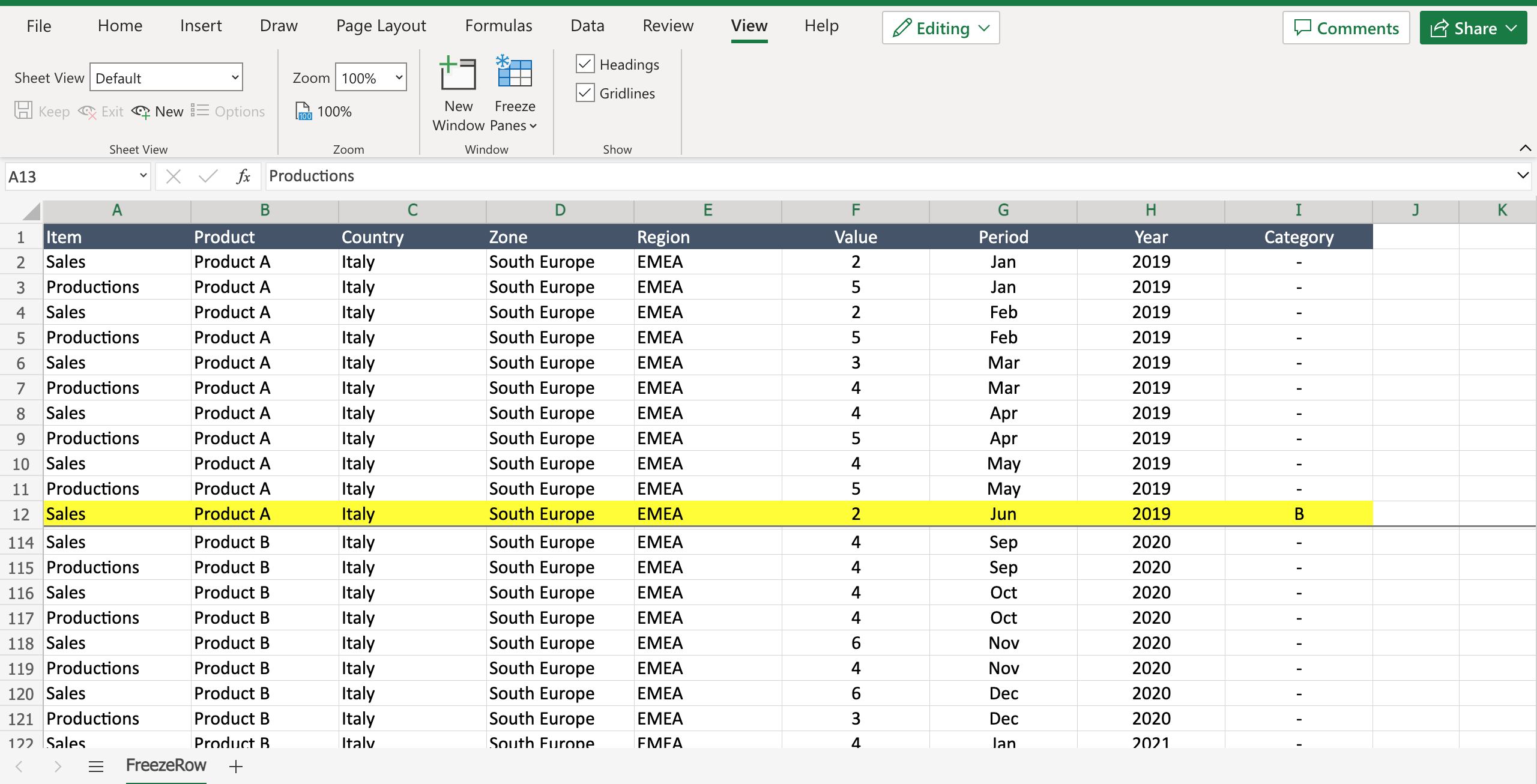
If you’re dealing with a huge amount of data and you have to continuously scroll down the page to see the info you need, you can use the freeze feature of Excel to keep a part of the data always visible while scrolling down the file. For Example if you have an important record at row 24 and you want to compare that record with the one in row 112, you can freeze row 24 to have it visible with row 114. To freeze a specific row in Excel proceed as follows.
Step 1 – Select the rows you want to freeze
– Click on the row number of the row just below the one you want to freeze.
Step 2 – Freeze the row
– Navigate to the “view” tab;
– Click on “freeze panes” icon to open the dialog menu;
– Select “freeze panes” to freeze the selected row.


