How to freeze a frame (Multiple Rows & Columns) in Excel

How to Freeze Single Row, Single Column and Panes (multiple rows & columns) in Excel

Microsoft Excel offers some very interesting features to handle large data sets. These features are very handy when we want to navigate through the data in an Excel workbook with a big data set, i.e. rows and columns of the order of 100s to 1000s. Some of these features are described below;

• Freeze top row (header row)
• Freeze first column (very first column with IDs or Names)
• Freeze panes (Multiple rows and multiple columns)

We’ll learn about each of these features step by step.

Freeze First (Top) Row:

Let’s get started with the first feature. This feature allows us to freeze the first row, i.e. the header row of an Excel Workbook. Normally the header row is very important and it contains information which helps us to identify the type of the data in each column. By making the header row static, we can scroll through the other rows of data while keeping the header row visible all the time. To do this yourself, please follow the steps described below;

Step 1 – Locate the View tab

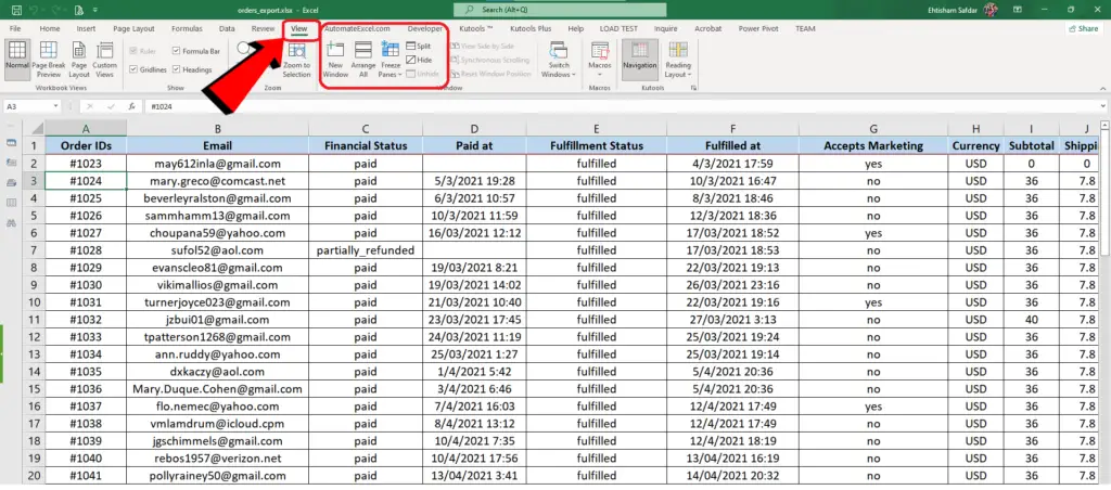
• Open the desired Excel workbook in which you want to enable this feature.
• Navigate to “View Tab” from the list of tabs available at the top row as shown;

Step 2 – Freezing the top row

• In “View Tab”, locate “Freeze Panes” and choose “Freeze Top Row” as shown below, and you are done. The first row is frozen now.

Freeze First Column:

To freeze the first column in an Excel workbook, the steps are pretty much similar to the previous one. However, to achieve this goal please follow the steps below;

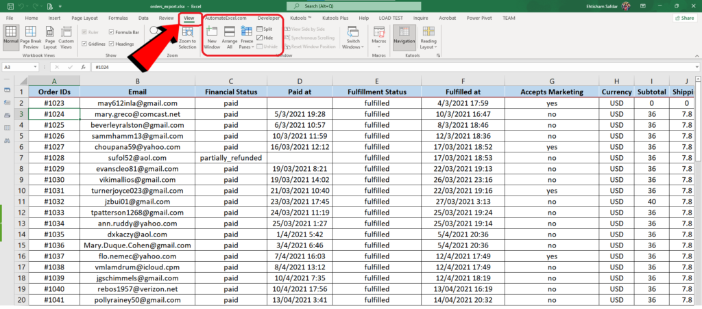
Step 1 – Locate the View tab

• Open the desired Excel workbook in which you want to enable this feature.
• Navigate to “View Tab” from the list of tabs available at the top row as shown;

 Step 2 – Freezing the first column

• In “View Tab”, locate “Freeze Panes” and choose “Freeze First Column” as shown below, and you are done. The first column is frozen successfully.

Freeze Panes:

This feature is very handy and useful when we want to freeze multiple rows and columns simultaneously. This is a little bit tricky as compared to the first two so please follow along the steps described below very carefully;

Step 1 – Locate the View tab

• Open the desired Excel workbook in which you want to enable this feature.
• Navigate to “View Tab” from the list of tabs available at the top row as shown;

Step 2 – Select the appropriate cell

• Now comes the tricky part, you will have to select a specific cell before activating this feature. The location of this specific cell will depend upon the following two things;
  1. Number of rows you want to freeze.
  2. Number of columns you want to freeze.

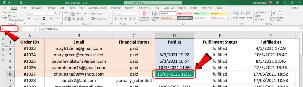
Let’s just say that you want to freeze the first five (5) rows and first three columns i.e. up to column C, then you will have to select the cell which lies just below the fifth (5th) row and next to the third column i.e. column C. So the location of the cell will be 6th row in Column D. The key cell is highlighted with green colour in the picture below to explain the procedure of cell selection.

Step 3 – Freeze Panes

• After selecting the cell as per the instruction given above,  you are all set to activate the feature to freeze the first five (5) rows & first three (3) columns. All you have to do is to go to “View Tab” again and in that tab locate the “Freeze Panes” option. This time we’ll use the very first option which is “Freeze Panes” also. This will activate our desired features and the first five rows and first three columns will be frozen successfully now. The procedure is also shown in the animated picture on the next page.