
How to freeze a formula in Excel
 By
SpreadCheaters
By
SpreadCheaters
You can watch a video tutorial here.
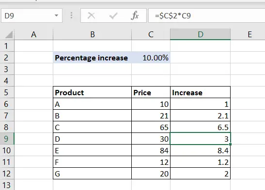
Excel is widely used for calculations and is very versatile when it comes to creating and copying formulas. When a formula is created using cell references, the cell references change when the formula is copied. If the formula is copied across rows then the row number changes accordingly and if it is copied across columns then the column letters change accordingly. Sometimes you will need to freeze a formula so that the cell references do not change when it is being copied. An example of this is when you have created a formula based on the value in a cell and the same value has to be applied to all rows in the column.
Step 1 – Create the formula
– Type the formula in the destination cell
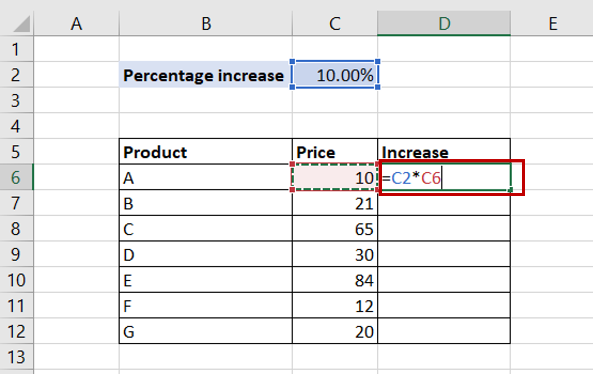
Step 2 – Freeze the formula
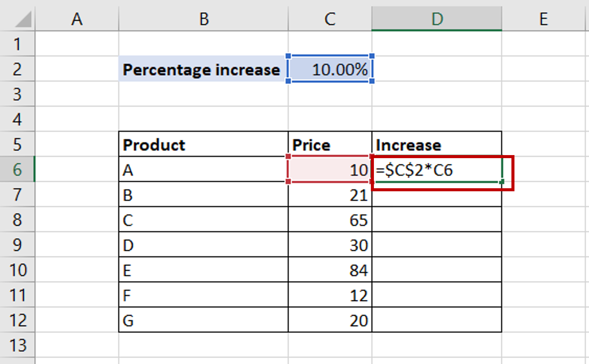
– Type dollar signs (‘$’) in front of the column name and the row number
– Alternatively, select the cell reference and press F4
Step 3 – Copy the formula to other cells
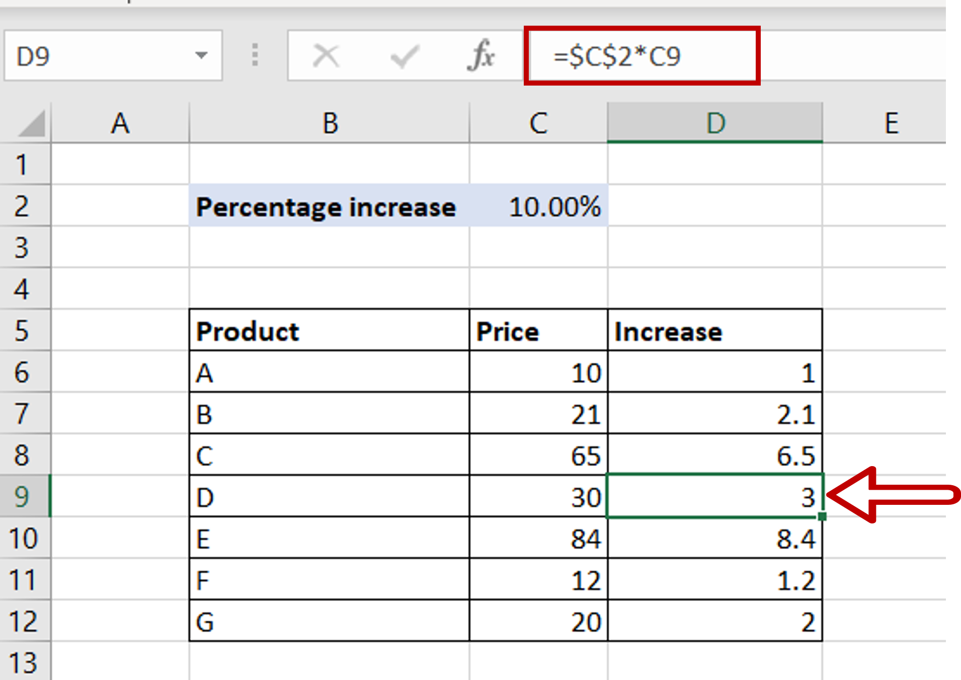
– Select the cell with the formula and press Ctrl+C or choose Copy from the context menu (right-click)
– Select the rest of the cells in the column and press Ctrl+V or choose Paste from the context menu (right-click)
– The cell C2 remains constant while the row number changes accordingly


