
How to format a phone number in Excel
 By
SpreadCheaters
By
SpreadCheaters
You can watch a video tutorial here.
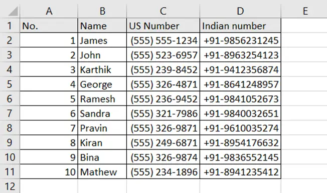
Excel is widely used for storing data and one piece of data that is common to a lot of databases is the phone number. To distinguish a phone number from any other numeric data, it is better to format it as a phone number. This makes the phone number easily recognizable. In this example, we will see how to use a preset format for a US phone number and how to define a format for an Indian mobile number.
Step 1 – Format the US phone numbers
– Select the column to be formatted
– Go to Home > Number and click on the arrow to expand the menu
OR
Right-click and select Format Cells from the context menu
OR
Go to Home > Cells > Format > Format Cells
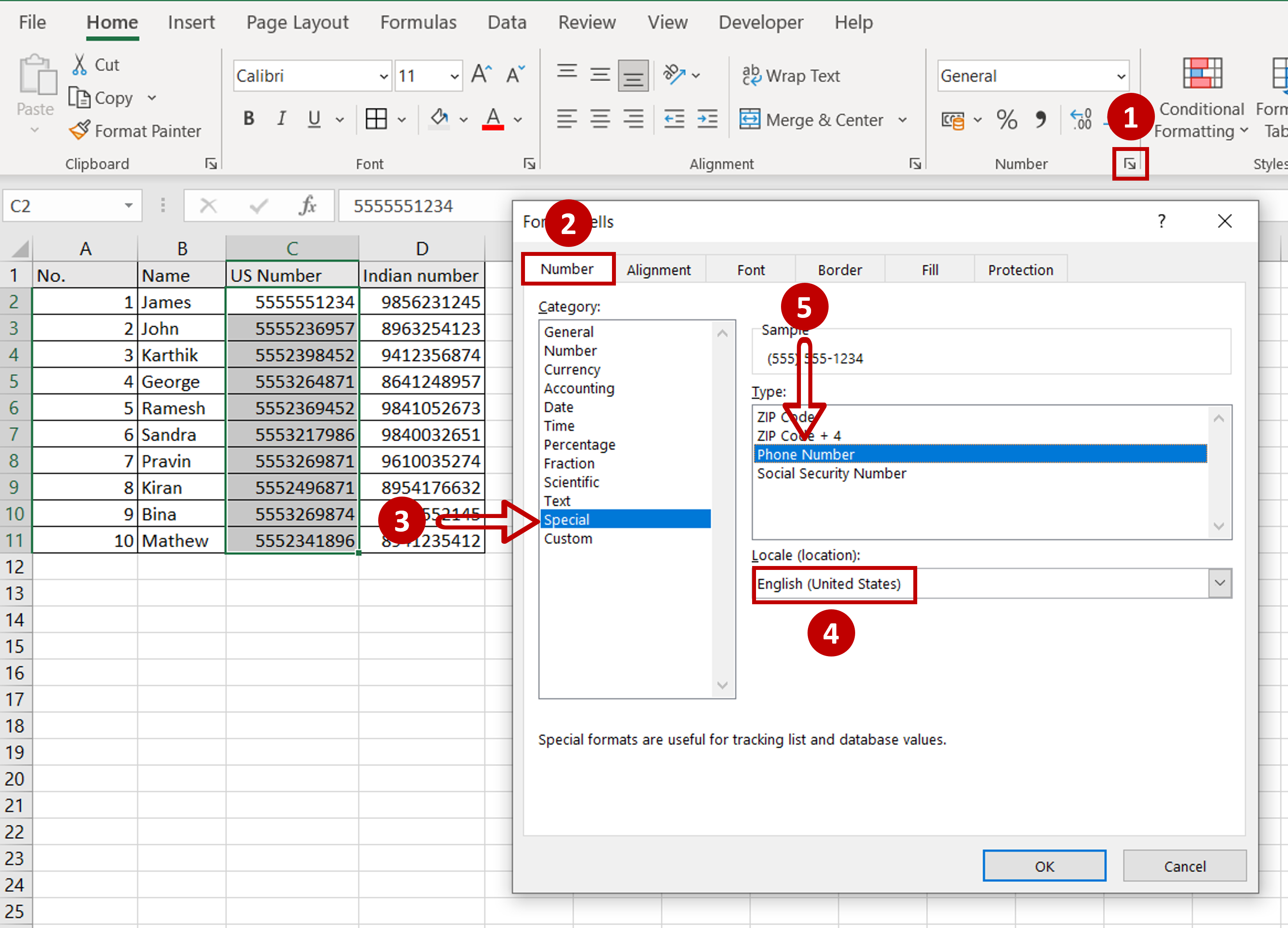
– In the Format Cells window go to Number > Special
– Select English (United States) as the locale
– Select Phone Number from the Type window
– Click OK
Step 2 – Format the Indian mobile phone numbers
– Select the column to be formatted
– Go to Home > Number and click on the arrow to expand the menu
OR
Right-click and select Format Cells from the context menu
OR
Go to Home > Cells > Format > Format Cells
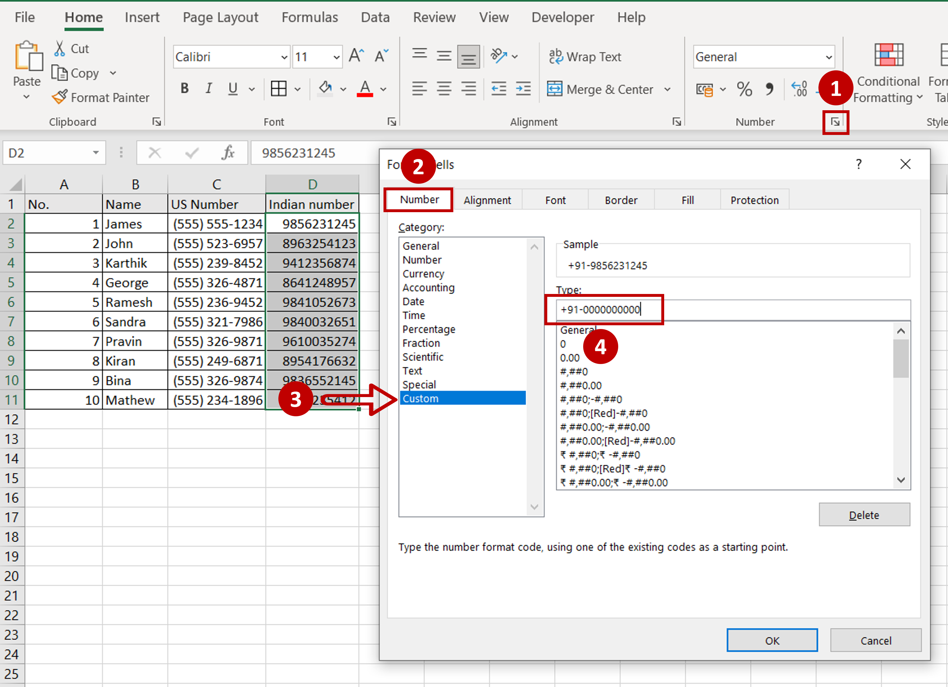
– In the Format Cells window go to Number > Custom
– Under Type enter: +91-0000000000
Note: +91 is the country code prefix for India and 10 zeroes represent the 10 digits of mobile numbers in India
– Click OK
Step 3 – Check the result
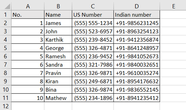
– The phone numbers have been formatted according to the country-specific format
– This method can be used to define custom formats for phone numbers for other countries as well


