
How to Flip Names in Excel
 By
SpreadCheaters
By
SpreadCheaters
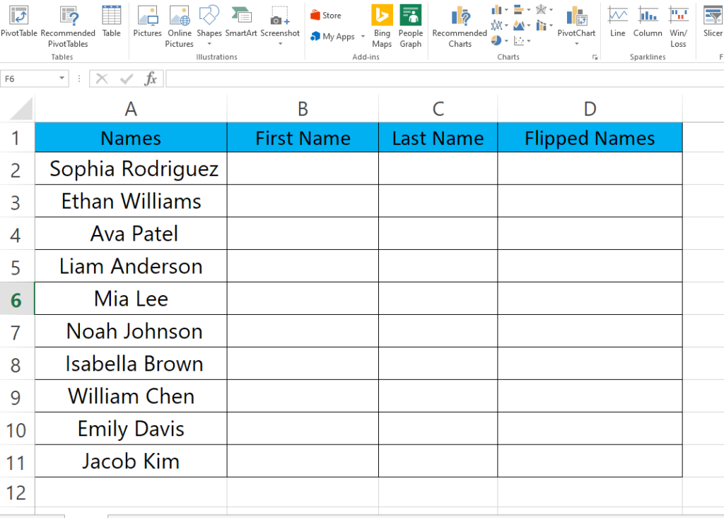
Here we have a dataset of ten random names, we will replace the first name with the last name and vice versa. Follow the steps below to do this but first we will have a look at the dataset above.
Have you ever needed to flip the order of names in an Excel spreadsheet? Whether you’re dealing with a long list of names or trying to organize data for a project, Excel makes it easy to switch the order of names with just a few clicks. In this tutorial, we’ll show you how to flip names in Excel.
Step 1 – Separate First and Last Names.
– To separate First and Last Names, select all the cells with names in it.
– Go to the DATA tab and open Text to Column in the Data Tools group.
– Click Next, Check the Space check box, click Next again.
– Type in the destination where the separated data will be shown, in our case it is B2.
– Then Click Finish.
Step 2 – Type the formula to Flip Names.
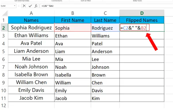
– Select the cell where you want to show the flipped names, in our case it is D2.
– Type in the formula, its syntax is
=Last_Name & “ “& First_Name
– In our case formula looks like this:
=C2&” ”&B2
Step 3 – Flip the rest of the Names automatically.

– Select the cell with formula.
– Drag the cell from bottom right to the last cell.
– Rest of the Flipped names will appear automatically.


