
How to flip data in Excel
 By
SpreadCheaters
By
SpreadCheaters
Page last updated:
18/11/2022 |
Next review date:
18/11/2024
You can watch a video tutorial here.

There are times when analyzing data that columns would be better expressed when they are displayed horizontally. The TRANSPOSE command is useful to convert the alignment of the data.
Step 1 – Highlight an empty array of cells

Highlight an empty array of cells
Step 2 – Type in the TRANSPOSE command in the formula bar

When using the TRANSPOSE command always select the cells that you need to change the orientation.
Step 3 – Press CTRL + SHIFT + ENTER
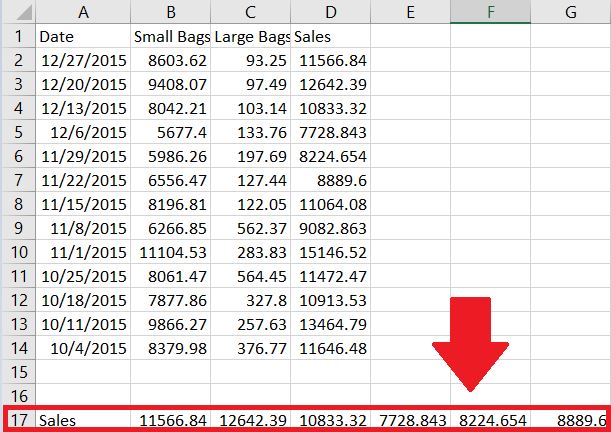
By pressing CTRL + SHIFT + ENTER the formula will return an array.It is important to note that the output of the transpose function is dependent on the highlighted cells. Since in this example, there are only 7 cells that have been highlighted, then only the same number of the selected data has been shown.


