
How to find the column index number in Excel
 By
SpreadCheaters
By
SpreadCheaters
In this tutorial we will learn how we can use Excel’s built-in functions to determine the column index number. The following methods can be used to determine the column index in Excel.
- COLUMN function
- CELL function
- MATCH function
The first two functions are very simple to use. However, the third function is a little different from the first two. We can find out the column index of a particular data column based on a criterion using MATCH function. It has the following syntax,
MATCH(lookup_value, lookup_array, [match_type])
lookup_value – The value to match in lookup_array.
lookup_array – A range of cells or an array reference.
match_type – [optional] 1 = exact or next smallest (default), 0 = exact match, -1 = exact or next largest.
Let’s see how we can use Excel’s built-in formulas to find a solution to our problem by following these steps;

In Microsoft Excel, a column is identified by a letter at the top of the column. For example, the first column is identified as “A”, the second column is “B”, and so on. The column index is the number that corresponds to the column letter. For example, the column index of column “A” would be 1, the column index of column “B” would be 2, and so on.
Step 1 – Use COLUMN function
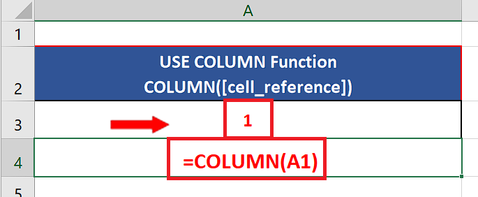
– Choose a suitable cell where you wish to implement the formula.
– Use the following formula in that cell and press enter key.
=COLUMN(A1)
– The desired result i.e., 1 will be displayed in this cell as soon as you press the enter key as shown in the picture below. Using this function, we can find out the column index of any cell in the sheet.
Step 2 – Use CELL function
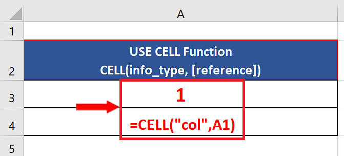
– Choose a suitable cell where you wish to implement the formula.
– Use the following formula in that cell and press enter key.
=Cell(“col”, A1)
– Using this function, we can find out the column index of any cell in the sheet. When cell function is used with “col” it gives us the column index of the reference cell as shown above.
Step 3 – Use MATCH function
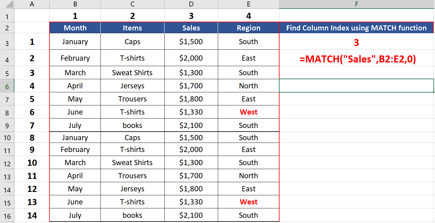
– We’ll see the following formula in a suitable cell to find the column index of “Sales” from the dataset used in the example below,
=MATCH(“Sales”,B2:E2,0)


