How to find pivot table in Excel 

A PivotTable is a powerful feature in Microsoft Excel that summarizes and analyzes large amounts of data quickly and easily. With pivot tables, you can quickly extract valuable insights from this data. For instance, you can create a pivot table to summarize the total sales by region, allowing you to compare the performance of each store location easily.

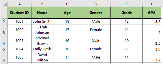
The dataset comprises a comprehensive set of records that pertain to a cohort of pupils. Each record corresponds to a specific student and furnishes valuable insights into their unique characteristics, such as their age, gender, academic standing, and grade placement. This dataset serves a range of purposes, from facilitating educational inquiry to assessing student achievement or monitoring progress over extended periods.

Method – 1 Using VBA code.

Step – 1 Open Visual Basic

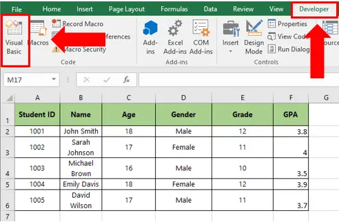
• Press the ALT + F11 keys, and it will open the Microsoft Visual Basic for Applications menu.
• Alternatively, you may go to the Developer option and click on Visual Basic a new window will be opened.
• Click Insert tab in the Visual Basic Editor and again click Module. This will insert a new module in the workspace where you can add the VBA code.

Step – 2 Add and Run the code.

• In the blank sheet type the following code 

Sub ListPivotsInfor() ‘Update 20141112     Dim St As Worksheet     Dim NewSt As Worksheet     Dim pt As PivotTable     Dim I, K As Long     Application.ScreenUpdating = False     Set NewSt = Worksheets.Add     I = 1: K = 2     With NewSt         .Cells(I, 1) = “Name”         .Cells(I, 2) = “Source”         .Cells(I, 3) = “Refreshed by”         .Cells(I, 4) = “Refreshed”         .Cells(I, 5) = “Sheet”         .Cells(I, 6) = “Location”         For Each St In ActiveWorkbook.Worksheets             For Each pt In St.PivotTables                 I = I + 1                 .Cells(I, 1).Value = pt.Name                 .Cells(I, 2).Value = pt.SourceData                 .Cells(I, 3).Value = pt.RefreshName                 .Cells(I, 4).Value = pt.RefreshDate                 .Cells(I, 5).Value = St.Name                 .Cells(I, 6).Value = pt.TableRange1.Address             Next         Next         .Activate     End With     Application.ScreenUpdating = True End Sub

Code Explanation is given at the end of the document.

• Now go to Run and run the code and all the pivot table names, source data range, worksheet name, and other attributes will be listed in a new worksheet which placed in the front of your active worksheet,

Method – 2 Find pivot tables using To Find option 

Step – 1 Open To Find dialogue box

• Open the Excel worksheet that contains the PivotTables you want to find.
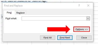
• Press the “Ctrl” and “F” keys simultaneously to open the “Find” dialog box.
• In the “Find” dialog box, click on the “Options” button to expand the options as shown.

Step – 2 Copy a cell formatting and find Pivot table 

• Click on the “Format” drop-down box and select “Choose Format From Cell“.
• Select any cell within a PivotTable on the worksheet to copy its formatting.
• Click on the “Find All” button.
• Excel will now list all PivotTables found on the worksheet in the “Find and Replace” dialog box.
• Double-click on any PivotTable in the list to select it on the worksheet.
• Repeat the process to find any other PivotTables on the worksheet.

Code Explanation:

Dim St As Worksheet: Declares a variable “St” of type Worksheet to represent individual worksheets in the workbook.

Dim NewSt As Worksheet: Declares a variable “NewSt” of type Worksheet to represent a newly added worksheet where the pivot table information will be listed.

Dim pt As PivotTable: Declares a variable “pt” of type PivotTable to represent individual pivot tables within each worksheet.

Dim I, K As Long: Declares variables “I” and “K” as Long data type. These variables will be used for tracking the row numbers in the new worksheet.

Application.ScreenUpdating = False: Disables screen updating to improve macro performance and prevent flickering.

Set NewSt = Worksheets.Add: Creates a new worksheet and assigns it to the “NewSt” variable.

I = 1: K = 2: Initializes variables “I” and “K” with values 1 and 2 respectively. These variables are used for tracking row numbers.

With NewSt: Begins a With statement for the “NewSt” worksheet.

.Cells(I, 1) = “Name” … .Cells(I, 6) = “Location”: Writes the column headers for pivot table information in the first row of the “NewSt” worksheet.

For Each St In ActiveWorkbook.Worksheets: Begins a loop to iterate through each worksheet in the active workbook.

For Each pt In St.PivotTables: Begins a nested loop to iterate through each pivot table in the current worksheet.

I = I + 1: Increments the row number in the “NewSt” worksheet for writing the pivot table information.

.Cells(I, 1).Value = pt.Name … .Cells(I, 6).Value = pt.TableRange1.Address: Writes the pivot table information to the respective cells in the “NewSt” worksheet.

Next: Ends the inner loop for pivot tables.

Next: Ends the outer loop for worksheets.

.Activate: Activates the “NewSt” worksheet.

Application.ScreenUpdating = True: Enables screen updating again.

End Sub: Ends the macro.

In summary, this VBA macro creates a new worksheet and lists information about pivot tables from all worksheets in the active workbook. The pivot table information includes the pivot table name, source data range, refresh name, refresh date, worksheet name, and table range address. The information is populated in the newly created worksheet, allowing for easy access and analysis of pivot table details.