How to find missing values in Excel.

Microsoft Excel is a powerful tool that is widely used for data analysis and management. However, working with datasets can sometimes be daunting, especially when dealing with missing values. Missing values can occur due to multiple reasons, such as human error, data entry issues, or technical problems. Fortunately, Excel provides several tools to help you find and handle missing values.

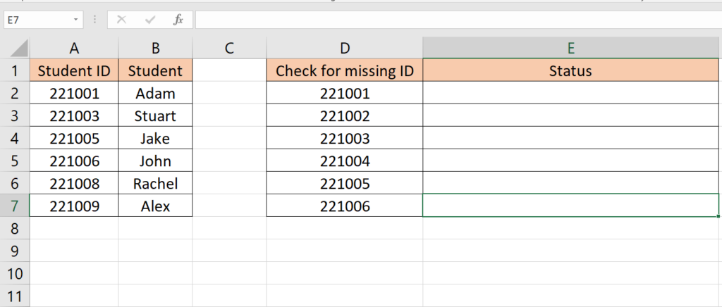
Here we have a dataset, in this dataset, we have two columns containing Student IDs and Student names. We have another column that we will use as a reference to find the missing values. In this tutorial, we will understand how to find missing values in Excel but first let’s take a look at the Dataset.

Method – 1 Using the Combination of IF and COUNTIF Functions.

Step – 1 Write the formula.

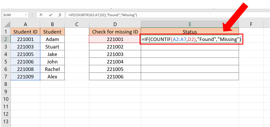
• Select the cell where you want to write the formula.
• The syntax of the formula will be

=IF(COUNTIF(Lookup_Array,Lookup_Value),”Found”,”Missing”)

• In our case the formula will be

=IF(COUNTIF(A2:A7,D2),”Found”,”Missing”)

• Formula explanation is given at the end of the document.

Step – 2 Find the values of the remaining cells.

• Press enter to apply the formula.
• Keep changing the Lookup_Value section to match the value you want to find.

Method – 2 Combining IF, ISNA, and MATCH Functions.

Step – 1 Write the formula.

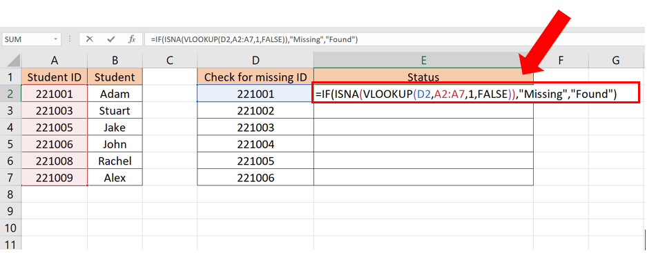
• Select the desired cell where you want to type the formula.
• The syntax of the formula will be

=IF(ISNA(VLOOKUP(Lookup_Value,Lookup_Array,1,FALSE)),”Missing”,”Found”)

• In our case the formula will be

=IF(ISNA(VLOOKUP(D2,A2:A7,1,FALSE)),”Missing”,”Found”)

• Formula explanation is given at the end of the document.

Step – 2 Find the values of the remaining cells.

• Press enter to apply the formula.
• Keep changing the Lookup_Value section to match the value you want to find.

Explanation of the formula:

Method 1 Formula:

=IF(COUNTIF(A2:A7,D2),”Found”,”Missing”)

IF: It is a conditional function that checks a logical condition and returns first value if the condition is true and second value if the condition is false.

COUNTIF: It is a function which counts the number of cells within a range that meet a specified criterion.

A2:A7: The range of cells in which to count.

D2: The criterion or value to count within the range.

“Found”: The value to return if the COUNTIF function counts any matching occurrences of the value in D2 within the range A2:A7.

“Missing”: The value to return if the COUNTIF function does not find any matching occurrences of the value in D2 within the range A2:A7.

So, the formula counts the occurrences of the value in cell D2 within the range A2:A7 using COUNTIF. If any occurrences are found, it returns “Found“; otherwise, it returns “Missing“.

Method 2 Formula: 

=IF(ISNA(VLOOKUP(D2,A2:A7,1,FALSE)),”Missing”,”Found”)

IF: It is a conditional function that checks a logical condition and returns first value if the condition is true and second value if the condition is false.

ISNA: It is a function that checks if a value is an #N/A error. In this case, it checks if the VLOOKUP function returns an #N/A error.

VLOOKUP: It is a lookup function that searches for a value in the first column of the range and returns a corresponding value from a specified column.

D2: The value to search for in the range.

A2:A7: The range where the value should be searched.

1: The column index from which the corresponding value should be returned (in this case, the first column).

FALSE: It specifies an exact match. The VLOOKUP function will return an #N/A error if an exact match is not found.

“Missing“: The value to return if the VLOOKUP function returns an #N/A error, indicating that the value was not found in the range.

“Found“: The value to return if the VLOOKUP function does not return an #N/A error, indicating that the value was found in the range.

So, the formula checks if the value in cell D2 is found in the range A2:A7 using VLOOKUP. If the value is found, it returns “Found”; otherwise, it returns “Missing”.