How to find duplicates in Excel between two columns

Finding duplicates in Excel between two columns can be a useful task when working with large datasets. Duplicates can occur when data is entered multiple times, or when data is imported from multiple sources. In this tutorial, we will explore two methods to find duplicates in Excel between two columns.

Here we have a dataset, in this dataset, we have two columns Column A and Column B which contain duplicates that we need to find. In this tutorial, we will learn how to find duplicates in Excel between two columns but first, let’s take a look at the Dataset.

Method – 1 Using Conditional Formatting.

Step – 1 Select the columns.

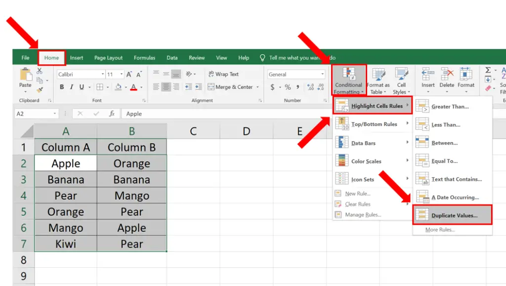
• Select the cells in both columns in which you want to find the duplicates.
• Click the Home tab in the Excel ribbon and select the Conditional Formatting command from the Styles group.
• From the drop-down menu, select Highlight Cell Rules and then click Duplicate Values.

Step – 2 Finding the duplicates.

• In the Duplicate Values dialog box, check if Duplicate is selected. 
• In the Values box and Light Red Fill with Dark Red Text is selected in the Format with box.
• Click OK to apply the formatting. 

Method – 2 Using COUNTIF Function.

Step – 1 Write the formula.

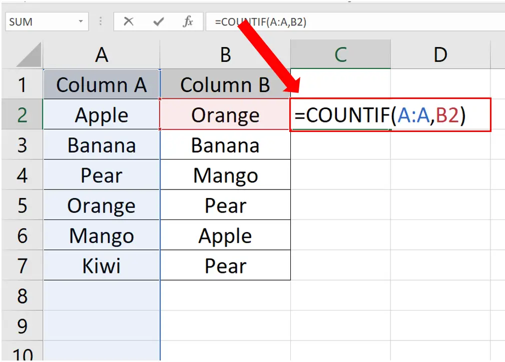
• Select a blank to write the formula.
• The syntax of the formula will be

=COUNTIF(First_Column_Range,Cell_In_Second_Column)

• In our case the formula will be

=COUNTIF(A:A,B2)

where A: A is the first column of data and B2 is the first cell in the second column of data.

Step – 2 Finding the duplicates.

• Press Enter to apply the formula to the cell.
• Drag the fill handle of the cell down to apply the formula down to the end of the column.
• Any cell with a value of 1 or greater indicates a duplicate between the two columns.

Method – 3 Using Equal operator.

Step – 1 Write the formula.

• Select a blank cell where you want to write the formula.
• The syntax of the formula will be

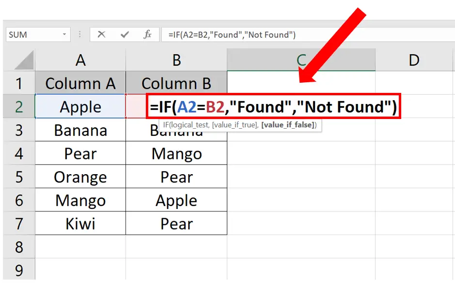
=IF(First_Cell_Address=Second_Cell_Address,”Found”,”Not Found”)

• In our case the formula will be

=IF(A2=B2,”Found”,”Not Found”)

Step – 2 Finding the duplicates.

• Press Enter to apply the formula to the cell.
• Drag the fill handle of the cell down to apply the formula down to the end of the column.

Method – 4 Using LookUp Function

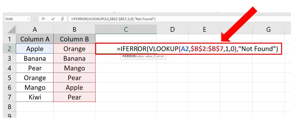
We can also use VLOOKUP to find the duplicates between two columns. In VLOOKUP, we will use the entries of fist column as the lookup keys and search them in the second column. If a match is found the matching name of the fruit will be shown, otherwise Not Found will be displayed. 

Step – 1 Write the formula.

• Select a blank cell  to write the formula.
• Syntax of the formula will be

=IFERROR(VLOOKUP(First_Column_Cell,Second_Column_Range,1,0),”Not Found”)

• In our case the formula will be

=IFERROR(VLOOKUP(A2,$B$2:$B$7,1,0),”Not Found”)

Step – 2 Finding the duplicates.

• Press Enter to apply the formula to the cell. 
• Drag the fill handle of the cell down to apply the formula down to the end of the column.
• The formula will be implemented and you’ll see that matching values with respect to the first column entries will be displayed when a match is found. In case of no match, “No Match” will be displayed as shown above.