
How to find duplicate rows in excel
 By
SpreadCheaters
By
SpreadCheaters
While working with large datasets users often face a situation in which duplicate values occur in many rows and they wish to find out the duplicate ones. The rows having exactly the same content in each column are called the duplicate rows.
To find and highlight the duplicate rows, we will use conditional formatting with custom formulas. Let’s see how we can do this.
Step 1 – Select a data range
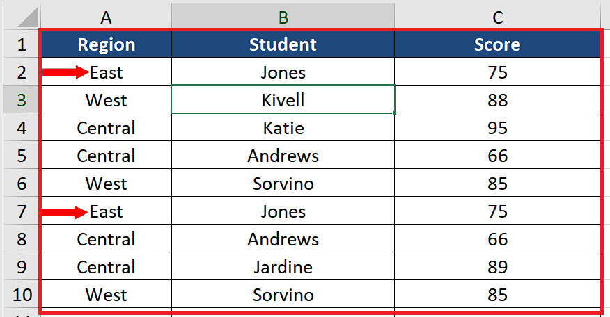
– With the help of handle select and drag to define the data range. One duplicate row is marked with arrows as an example.
Step 2 – Go to Home tab
– Now go to the Home tab.
Step 3 – Go to Styles group
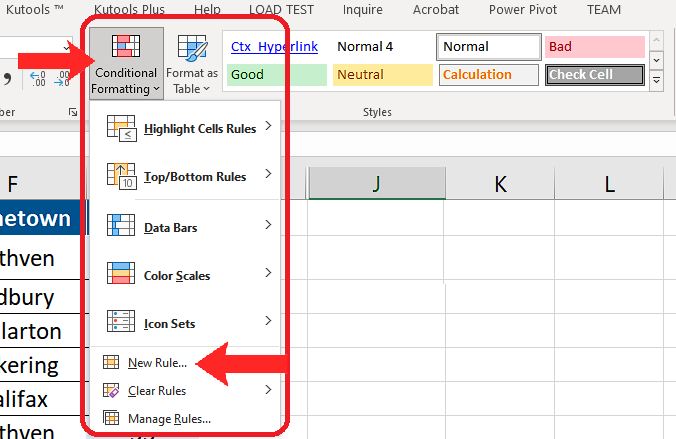
– Now go to the Styles group -> Conditional Formatting -> New Rule.
Step 4 – Write the appropriate formula to do conditional formatting
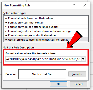
– Write the following formula in the conditional formatting formula bar;
=COUNTIFS($A$2:$A$10,$A2, $B$2:$B$10,$B2, $C$2:$C$10,$C2)>1
We have used COUNTIFS on each column of data to find out the exact duplicate rows. This function returns a TRUE when an exact match of all values in the columns of a row (say row 2) is found in the data range. Conditional formatting will highlight the duplicate rows when the condition is true.
Step 5 – Set the format for conditional formatting
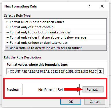
– Click on the format tab so that we can choose formatting styles to highlight our data range.
Step 6 – Set the font to bold for conditional formatting
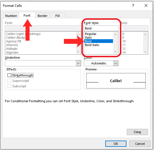
– In the next dialog box, click on the Font tab and select Bold.
Step 7 – Set the suitable colour for conditional formatting
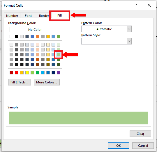
– In the same dialog box, click on the Fill tab and select an appropriate colour for highlighting the data.
Step 8 – Finalize and apply the conditional formatting settings

– When you click on the OK button in the last step, you will see another window.
– Click on OK again and this will implement the conditional formatting. The duplicate rows will be highlighted with the suitable colour.


