
How to filter rows in Excel
 By
SpreadCheaters
By
SpreadCheaters
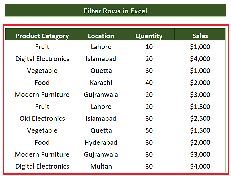
In today’s tutorial we are going to learn how to Filter Rows in Excel. Let’s take a look at the following sales dataset.

Microsoft Excel is one of the best tools which is simple to use yet it provides so many features to handle, manipulate and perform simple to complex calculations on any type of dataset. It also provides many built-in tools and features that can help the data analysts in visualizing data in the best possible ways. One such feature is the ability of Excel to apply filter on datasets to temporarily hide the unwanted information.
Step 1 – Apply the filter using shortcut key CTRL+SHIFT+L

– Select a cell inside your dataset.
– Use the shortcut key to apply a filter to the dataset by pressing CTRL+SHIFT+L.
– This will apply the filter to all columns in the data range automatically.
– The same thing can also be done by going to the Sort & Filter option in the Editing group on the Home tab from the list of main tabs in Excel.
Now that we have applied the filter to our data, we can use it as per our requirements to see only the data that we are interested in. Let’s assume that we wish to see the sales data of Fruit items only from the Product Category column. So, let’s use the filter options to get it done.
Step 2 – Use Filter options to filter rows in Excel
– We’ll go to the column header of interest, which in our case is the Product Category and click on the dropdown arrow.
– This will open up new options and we will see that all items are selected. Uncheck Select all option to exclude all items.
– Now select only the specific item you want to see, and in our case, it is Fruit. So we’ll select Fruit which will display all rows of data which include Fruit.
Step 3 – Clear filter from the data
– We can clear the filter applied in the previous step by clicking again on the drop down and then clicking on the Clear Filter From “Product Category” option.
– This will clear the filter and all data will be shown again.
If we are applying the filters to a column of data that contains only Text Data then we’ll see a choice of applying text filters as well. There are a lot of options in this area which can be used as per requirements. Let’s see how to do it in the step below.
Step 4 – Choose an appropriate filter from Text Filters options
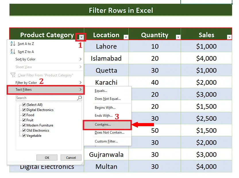
– To apply a text filter, go to the Product Category column and again click on the drop-down arrow.
– From the options available, click on the Text Filters and then choose whatever filter that suits your requirement. In our case we’ll choose “Contains” option.
Step 5 – Fill in Contains Filter options appropriately
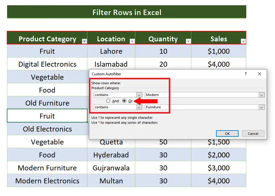
– The last step will open up a Custom Filter dialog box with some options. You may fill in the options as per your requirements. However, we’ll search for all those items which either have Modern or Furniture in their description. So, fill in the options as shown in the picture above.
Step 6 – Apply the Text Filter conditions to filter rows
– After filling in the options properly, click the OK button.
– This will filter the data and we’ll get the rows, which either contain the word Modern or Furniture.
We can do the same thing with numeric data as well. If we select a column that contains only numeric data then we can apply the Number Filters on that data in pretty much the same way discussed above.


