
How to filter a pivot table by value
 By
SpreadCheaters
By
SpreadCheaters

In this tutorial, we will learn how to filter a pivot table by a specific value. For this purpose, we’ll use the dataset consisting of the names of students that are shown along with their marks in a pivot table. Now we’ll filter the names and marks of students who scored over 70. For this, we will use Filter by Value option. The following steps will guide you to use this option.

Filtering a pivot table by value means restricting the data displayed in the pivot table based on specific criteria or values. Filtering a pivot table by value is an important tool for data analysis, as it allows you to focus your attention on the most important data points and gain deeper insights into your data.
Step 1 – Click on the arrow
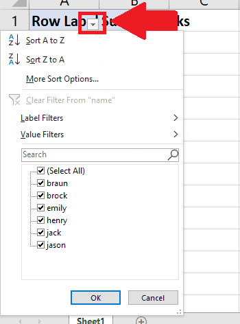
– In the pivot table, click on the arrow called Column label Filter in the first cell of the table and a drop-down menu will appear
Step 2 – Click on Value Filter

– In the dropdown menu, Click on the arrow next to the Value filter option and a right-side menu will appear
Step 3 – Click on the Greater Than option
– In the right side menu, Click on the Greater Than option and a dialog box will appear
– You can select any other option
Step 4 – Select the Value
– In the dialog box type the value (greater than which you want the values to be shown) in the third box and click on Ok to get the required result
– You can type any value according to your selected condition


