
How to fill color in Excel cell using if formula
 By
SpreadCheaters
By
SpreadCheaters
Here we have a dataset, in this dataset, we have two columns containing Student Names and their Test Score. In this tutorial, we will learn to fill color in an Excel cell using an IF formula and conditional formatting but first, let’s take a look at the DATASET.


Conditional formatting is a tool in Excel that is used to format cells based on a specific condition or criteria. One of the most common formatting options is to fill a cell with a color based on a specified condition.
Step – 1 Select the cells to fill.
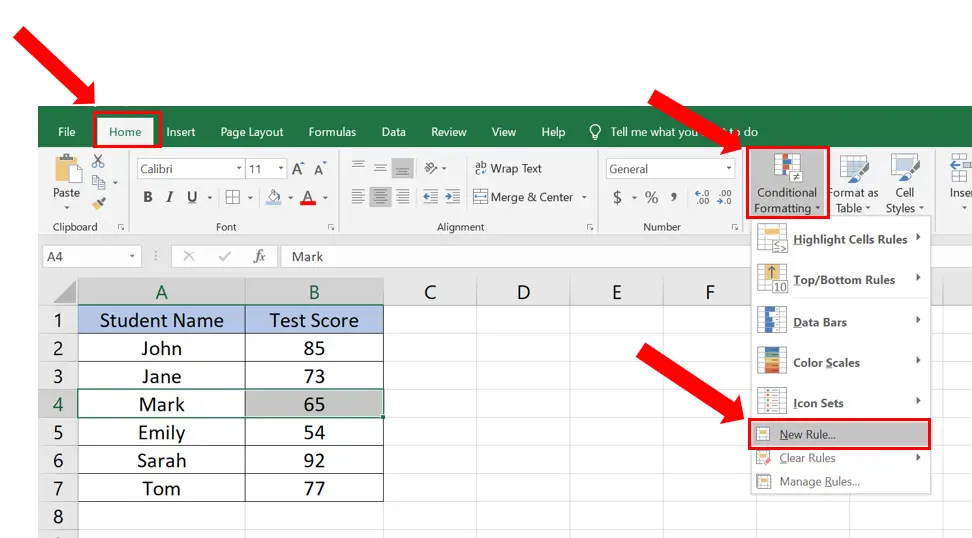
– Select the cell range you want to fill.
– Go to the Home tab in the Excel ribbon and select Conditional Formatting.
– Then click on New Rule.
Step – 2 Type the formula.
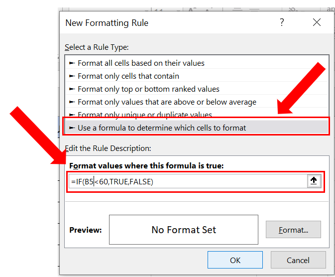
– In the New Formatting Rule dialog box, select Use a Formula to determine which cells to format.
– In the Format values where this formula is a true field, type the formula.
– In our case we will use the formula;
=IF(B5<60,TRUE,FALSE)
– If the value in cell B5 is less than 60, the formula will return the logical value “TRUE”.
– If the value in cell B5 is greater than or equal to 60, the formula will return the logical value “FALSE”.
Step – 3 Select the color.

– Click on the Format button and go to the Fill tab.
– Select the suitable color to apply to the cell and click OK.
– Click OK again to close the New Formatting Rule dialog box.


