
How to fill color in an Excel cell using a formula
 By
SpreadCheaters
By
SpreadCheaters
You can watch a video tutorial here.
Excel has several options for formatting cells and one such option is Conditional formatting. Using this, you can define the color of a cell based on its value. The value can be static or it can be based on a formula.
Step 1 – Open the New Formatting Rule window
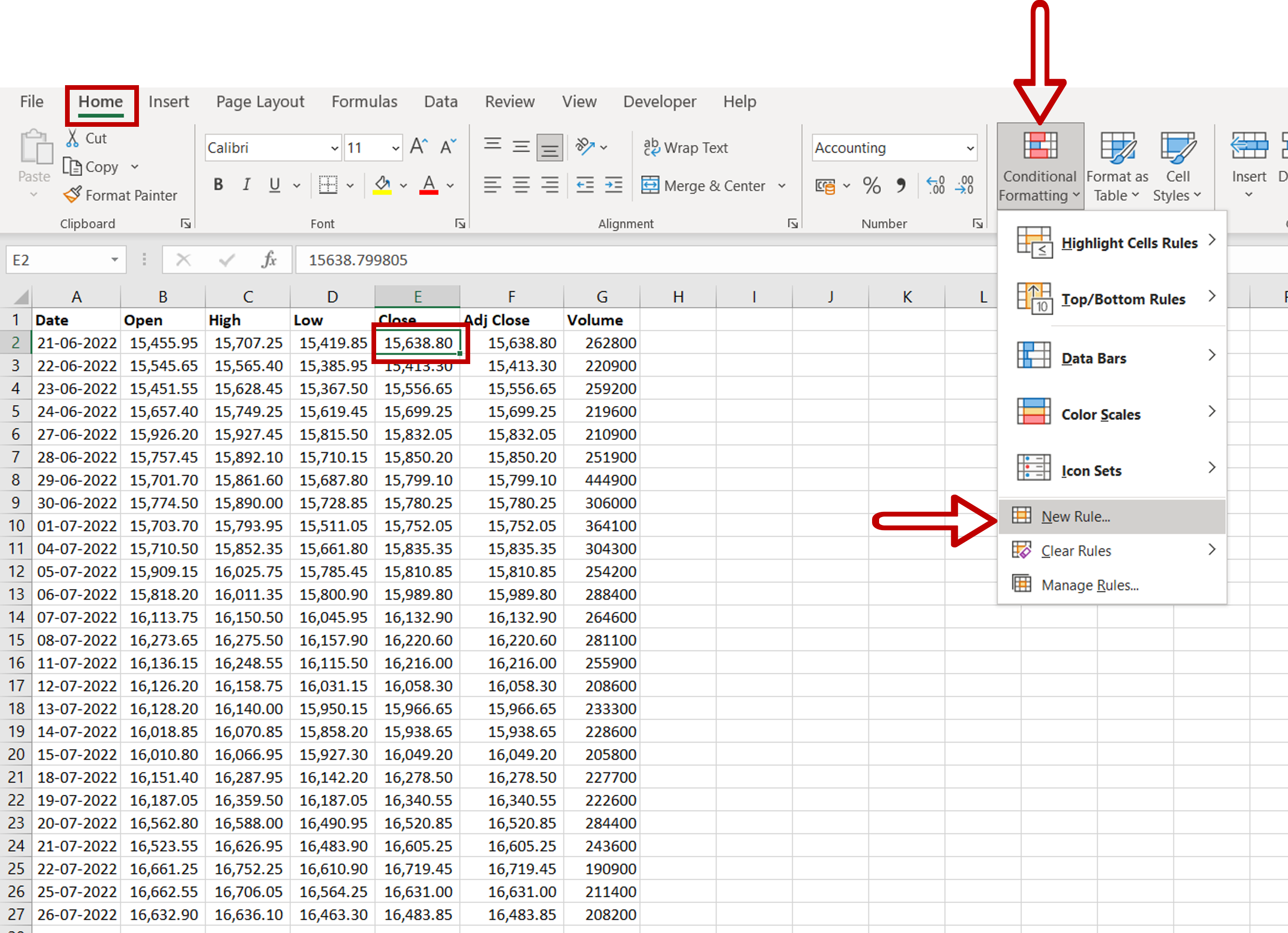
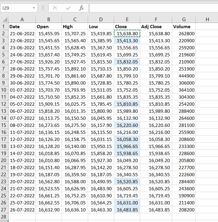
– Select the cell to be formatted
– Go to Home > Styles > Conditional Formatting
– Select New Rule
Step 2 – Create the formula
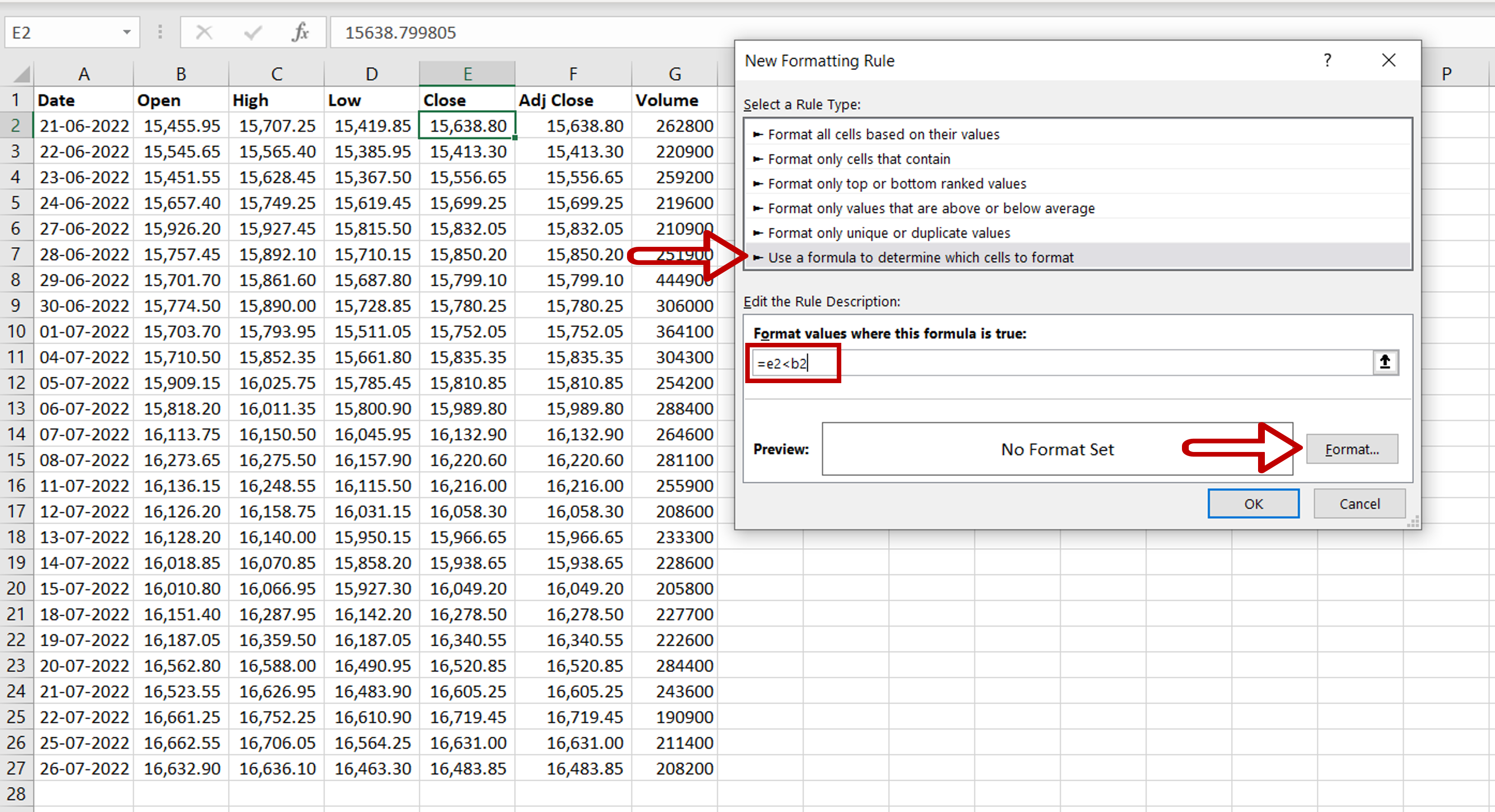
– Select Use a formula to determine which cells to format
– Type the formula using cell references:
= Close<Open
– Click Format
Step 3 – Choose the fill color
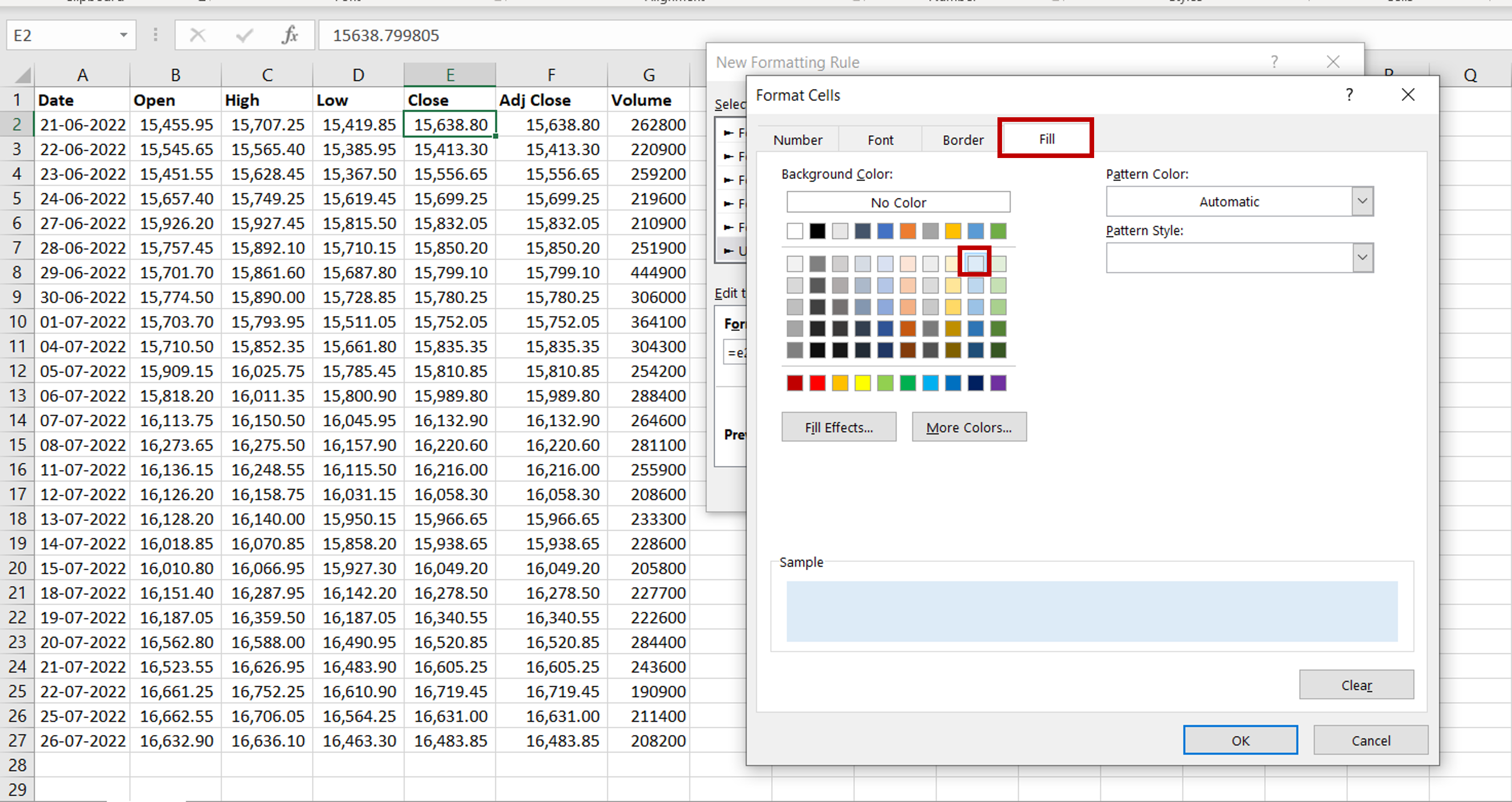
– Select the Fill tab
– Choose the color
– Click OK to close the Format Cells window
– Click OK to close the New Formatting Rule window
Step 4 – Copy the formula to the rest of the cells
– Copy the cell with the conditional formatting
– Select the rest of the column
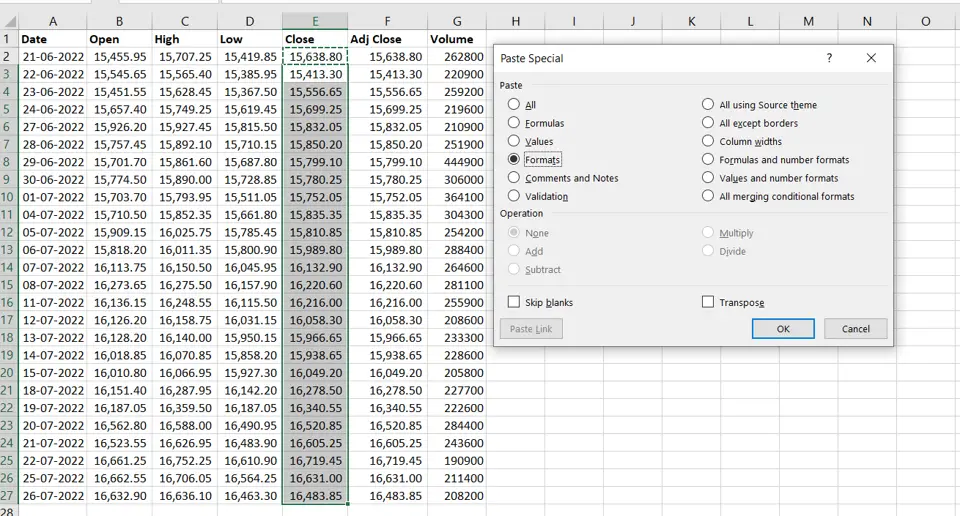
– Open the Paste Special window by right-clicking and selecting Paste Special from the context menu
OR
Go to Home > Clipboard > Paste > Paste Special
OR
Press Alt+E+S
– Select Formats
– Click OK
Step 5 – Check the result
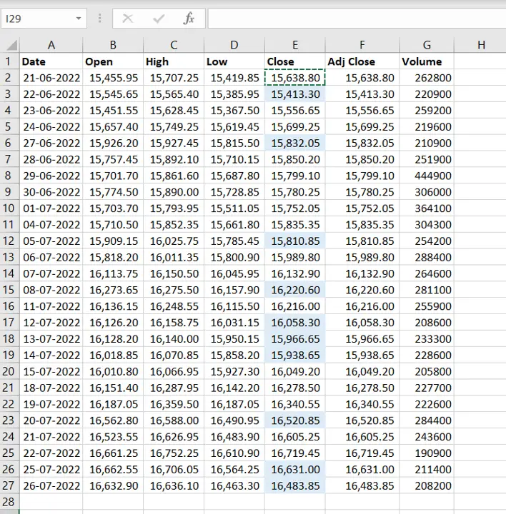
– The formatting has been applied to the cells


