How to extract the numeric portion of a street address in Excel

Microsoft Excel provides many features to handle the text data along with numeric data. There are many functions available to join, split and merge data in Excel. The data could be text only, numeric only or it could be alphanumeric as well. Sometimes, while working with city addresses, we need to split up the addresses for the sake of ease to understand the addresses better or to distinguish the addresses from each other. The numeric portion of a street address is important because it helps to identify a specific location within a city or town. This is particularly important in larger cities where there may be multiple streets with the same name. The numeric portion of the address, also known as the street number or house number, helps to distinguish one address from another on the same street.

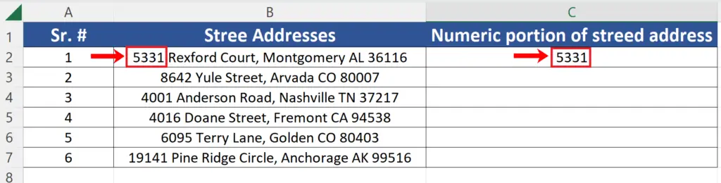
In this tutorial we’ll learn how to extract the numeric portion of a street address in Excel. Let’s look at the dataset above, it has records of street addresses and one sample address has been extracted manually to show what is required.

There are lots of methods in excel to do it.

• Use the Flash Fill 
• Use the LEFT with FIND function

Let’s explore each method one by one

Method 1: Using the flash fill

Step 1 – Create a sample and then use flash fill

• To use flash fill effectively, we need to make sure that our dataset is consistent and it doesn’t have any blanks in it, otherwise flash fill will work incorrectly.
• As we need the first numeric portion of the data so we’ll write 5331 in the target cell where we wish to extract the numeric portion.
• Now simply press CTRL+E and you will notice that it worked like a charm and all street numbers are extracted properly as shown above.

Method 2: Using LEFT and FIND functions together

Let’s discuss the functions’ syntax briefly to understand how to use these functions to get our goal.

Syntax of FIND 

Following is the syntax of the function 

FIND(find_text, within_text, [start_num])

This function searches the substring within a text string and returns its index inside the string. Here is the detail of the arguments that are required

find_text – It is the substring to find from the original text. 

We’ll use “ ” i.e., a blank because we wish to know the position or index number where the first blank appears in our street address. Our desired number finishes just before the first blank. The output of this function will be used as input for LEFT function.

within_text – This argument represents the text to search within. 

We’ll use B2 for the first formula and then keep on changing it by using non-absolute cell references. 

start_num – [optional] The starting position in the text to search. Optional, defaults to 1.

Syntax of LEFT

The syntax of LEF function is

=LEFT(text, [num_chars])

This function returns the number of characters from the left i.e., the beginning of the string. The details of arguments are as follows;

text – The text from which to extract characters. 

This will be our complete street address i.e., B2 for the first instance and then we’ll keep on changing it.

num_chars – [optional] The number of characters to extract, starting on the left side of text. Default = 1. 

This is the key argument. We’ll use the output of FIND function here as the second input argument. The FIND function will return us the index of the first blank space and we know we have to extract all data before that so we’ll subtract 1 from the index of first space.

The LEFT function will do the rest and extract the numbers for us as shown in the following steps.

Step 1 – Create and implement the formula using LEFT and FIND

• We’ll use the following formula;

=LEFT(B2,FIND(” “,B2)-1)

This will get our desired data in the cell C2 as shown above.