How to extract text after a character in Excel

Sometimes, while working with a team, you might get a spreadsheet in which the rows are separated by a comma. If you have to clean that data and write them into separate columns then doing that manually may take a lot of time and effort too.

In today’s tutorial we’ll learn how to handle such a dataset and split the data into different cells by using the delimiter. Let’s take a look at the following dataset.

 Excel provides three methods to achieve the goal

• Using the Flash Fill (CTRL+E) trick
• Using built-in Data Tool “Text to Columns”
• Using “Power Query”

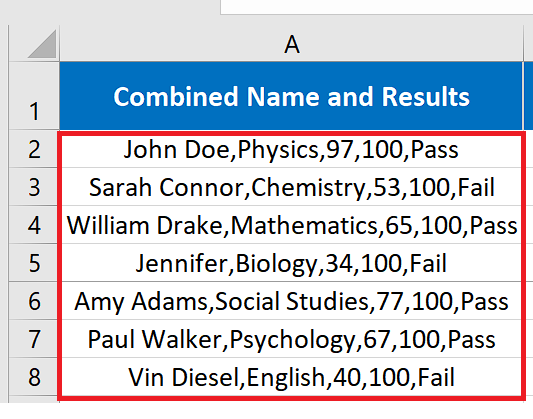
We can see that the dataset has Student Names, Subject Name, Marks obtained, Total Marks and Final results all in one cell separated by a comma only.

Method 1 – Using the Flash Fill Trick

In this method we are going to use Excel’s magical shortcut CTRL+E trick to flash fill the required data. Flash fill basically works using Excel’s built-in AI Engine, which recognizes the pattern in the data sets and then fills the whole data range using the same pattern. However, for this to work the data needs to be consistent in the pattern.

Step 1 – Create one sample of data to be extracted

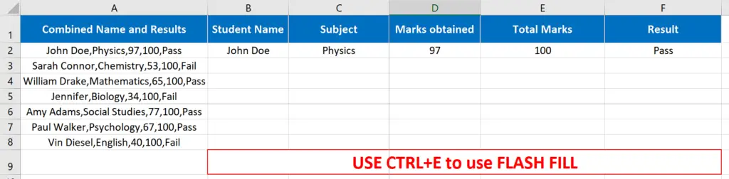
• We’ll create one example of the data point to be extracted so Excel can recognize that we wish to extract the email addresses after comma “,” from our data set.

Step 2 – Use CTRL + E to extract the required data

• After creating one example of the data point to be extracted, Excel is now ready to recognize the pattern and can extract required data from our data set by just using one simple command i.e. CTRL+E (Flash Fill). In this method the original data will remain intact.

Method 2 – Using the Data Tools “Text to Columns”

This method is also very handy and it can split the text data into different columns and we can choose any special character from “Tab”, “Semi colon”, “Comma”, “Space” and any other special character of our choice as well. Let’s dive into it and see how it can be done.

Step 1 – Select all the data set

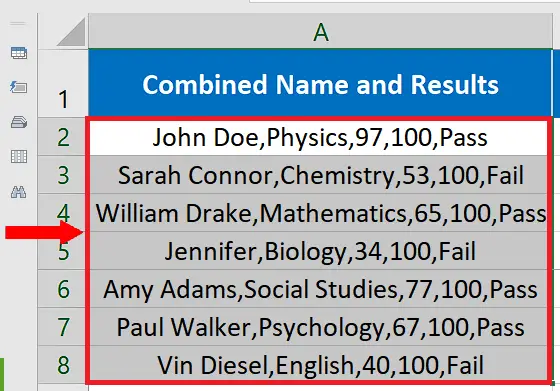
• We’ll use the same data set as before, so just select all the data containing names and email addresses.

Step 2 – Locate the Text to Columns Option on Data Tools

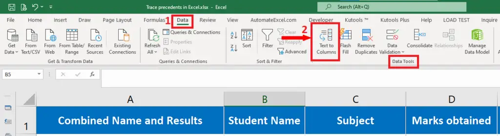
• On the Data tab, go to the Data Tools group and locate the Text to Columns option.

Step 3 – Choose appropriate data type

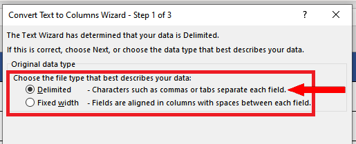
• Click on the “Convert to Columns” option and a new dialog box will open up. It will ask you to choose the data type. Since our data is delimited with commas, we’ll select the “delimited” option.

Step 4 – Choose the Data Delimiter

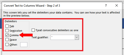
• Click on the “Next” option and we’ll reach 2 out of 3 to split up the data. 
• It will ask you to choose the data delimiter. Since our data is delimited with commas, we’ll select the “Comma” option.

Step 5 – Choose Output Format and Destination

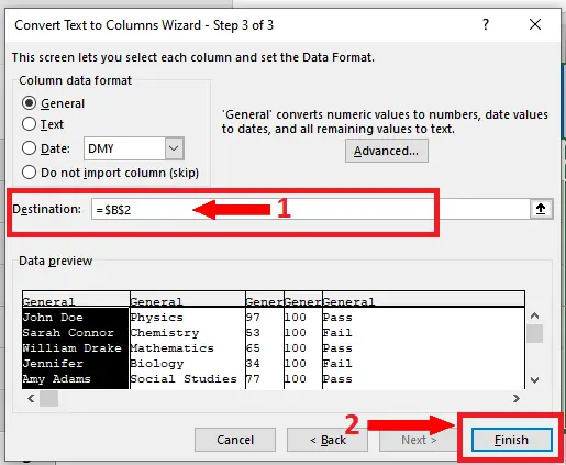
• In the last step 3 of this wizard to split up the data choose the output format and destination’s first column. 

Step 6 – Split Data cells separated by commas in different cells

• As the final step, just click the Finish button and you will get the data starting from the column that you chose in the last step.

Method 3 – Using the “Power Query” to split cells

Just like the second method, it is also very handy and it can split the text data into different columns and we can choose any special character from “Tab”, “Semi colon”, “Comma”, “Space”. Let’s dive into it and see how it can be done.

Step 1 – Load the data from Excel File

• Open a blank Excel spreadsheet.
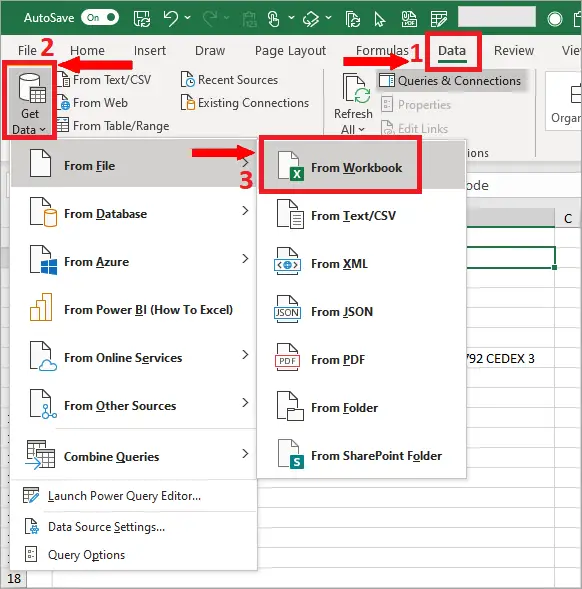
• Go to the Data tab on the list of main tabs and in the Get Data dropdown, locate the option of From File —> From Workbook as shown above.

Step 2 – Select the Excel File with data

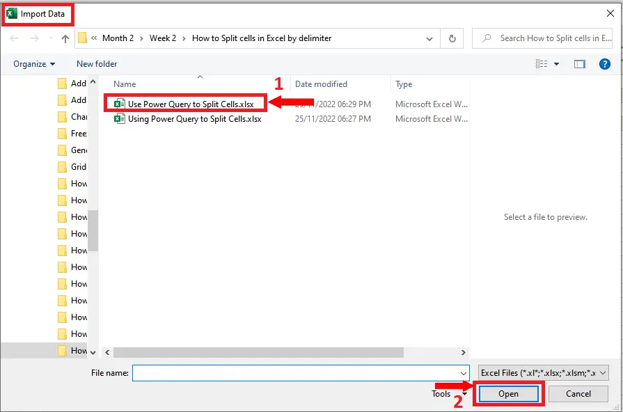
• This will open up the windows file selection dialog box.
• Browse to the required data file.
• After choosing the required data file press the Open button as shown above.

Step 3 – Select the worksheet tab in the selected Excel File

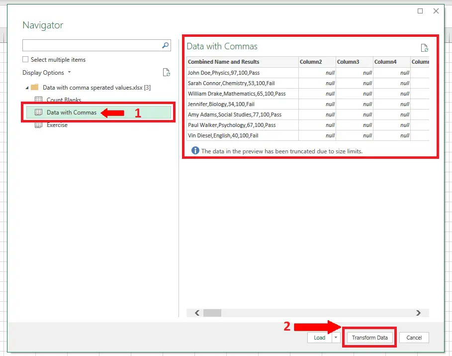
• Pressing Open in the last step will load the Excel file in Power Query Navigator.
• All available sheets inside the selected Excel file will be shown on the left side.
• Now choose the sheet which has the data to be splitted in Power Query Navigator and click on Transform.

Step 4 – Locate the Split Column and By Delimiter option

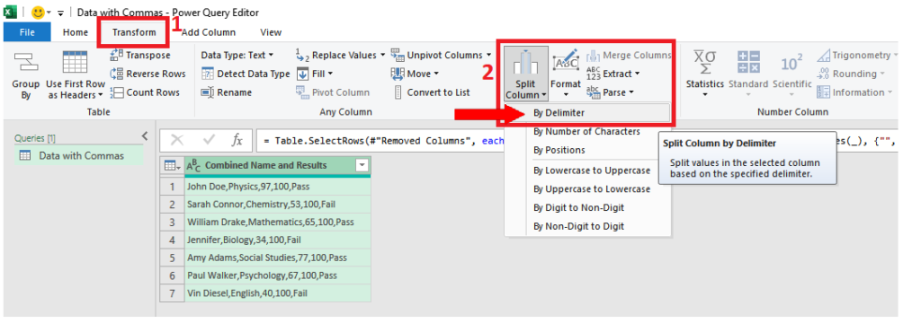
• The last step will load data and open up the Power Query Editor.
• Click on the Transform tab and then in the Split Column dropdown select By Delimiter as shown above.

Step 5 – Choose the Delimiter type and other options

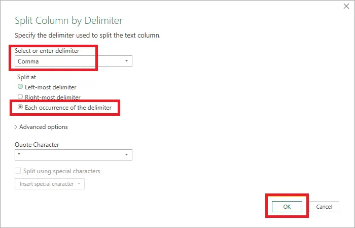
• Now a new options page “Split Column by Delimiter” will appear.
• Choose “Comma” in the “Select or enter delimiter” option.
• Choose “Each occurrence of the delimiter” in the “Split at” option and press the OK button.

Step 6 – Split the data separated by commas

• Now press the OK button and this will show you the preview of the data in Power Query Editor. It will split the cell into three new columns instead of one column.
• Now click on the “Close and Load” option. This will load the data in Excel as shown below and hence our data will be splitted as per our requirements.