
How to extract data from Excel based on criteria
 By
SpreadCheaters
By
SpreadCheaters
You can watch a video tutorial here.
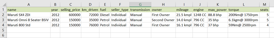
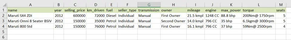
In Excel, filters are a popular way of extracting data to analyze it or to perform data cleaning operations. As long as the data is organized in columns, the filter can be applied to any column, even if the column does not have a header. To extract data you need to specify one or more criteria and only the rows that match those criteria are displayed. The rows that do not match the results are hidden. When you remove the criteria, all the rows are displayed again. In Excel, you can create in-column filters to filter and extract data. In this example, we will extract a list of all Maruti cars from 2012.
Step 1 – Enable the in-column filters
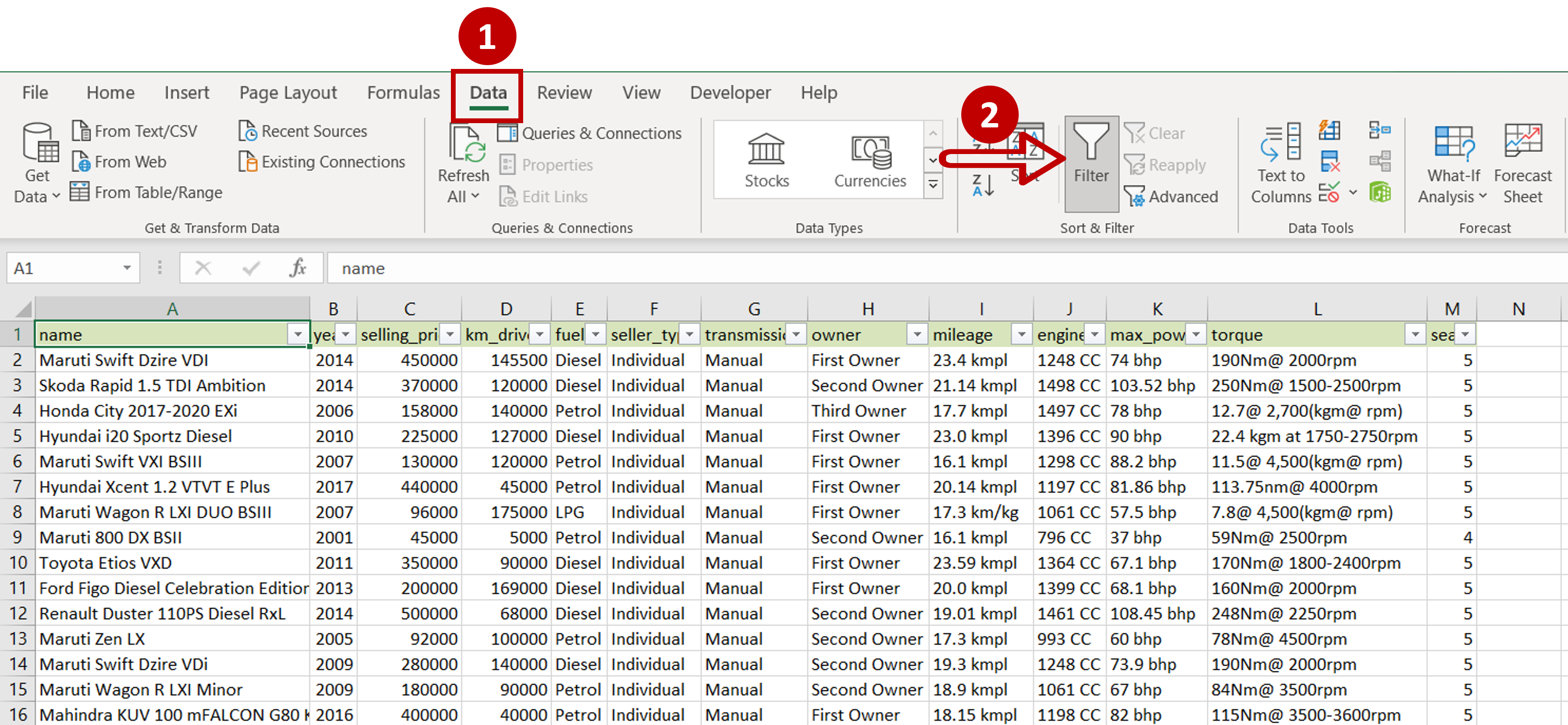
– Go to Data > Sort & Filter
– Click the Filter button
Step 2 – Apply the first condition
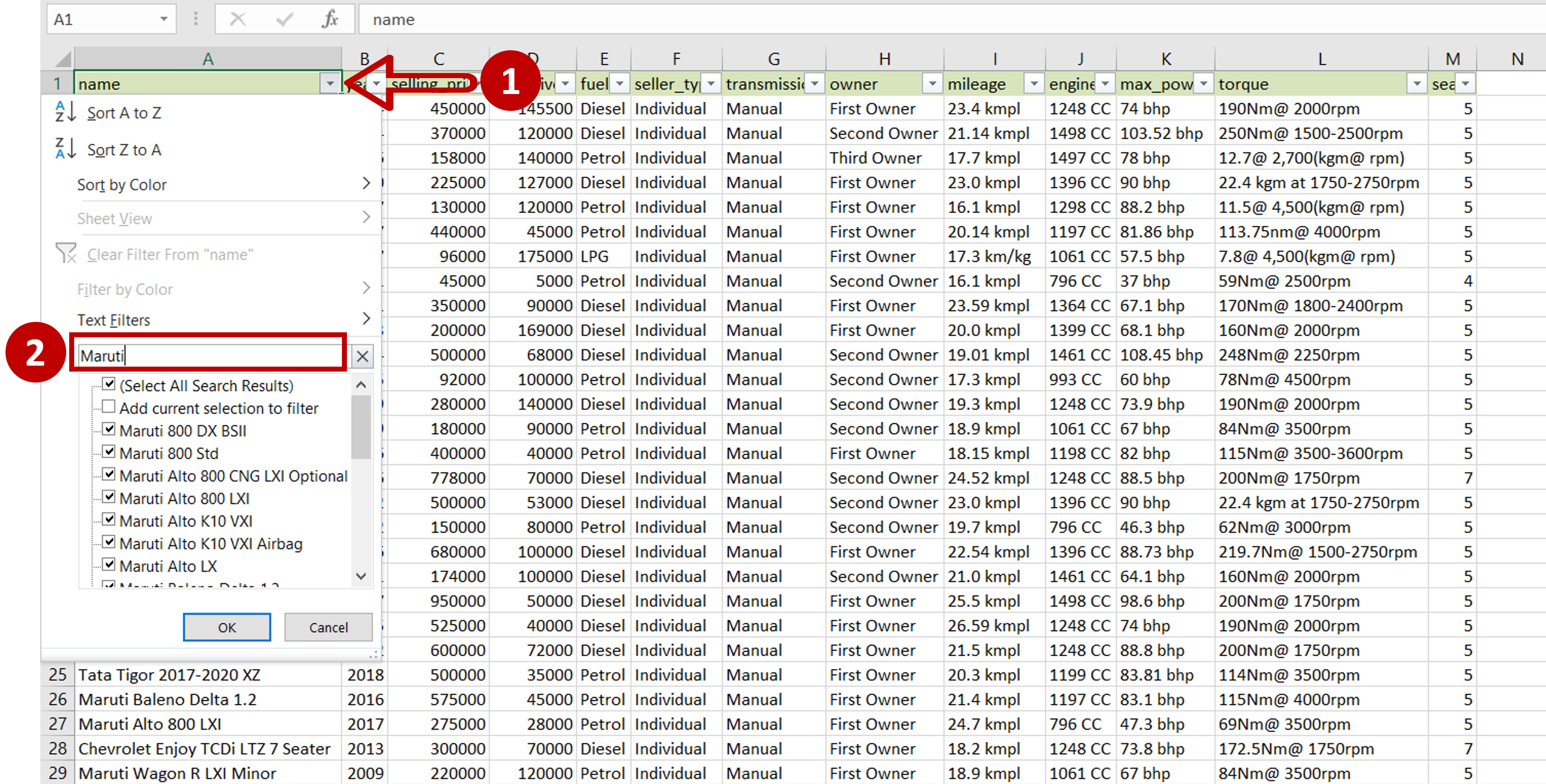
– Click the filter button in the ‘name’ column
– In the search box type: Maruti
– All values that start with ‘Maruti’ are displayed in the box
– Click OK
Step 3 – Check the list
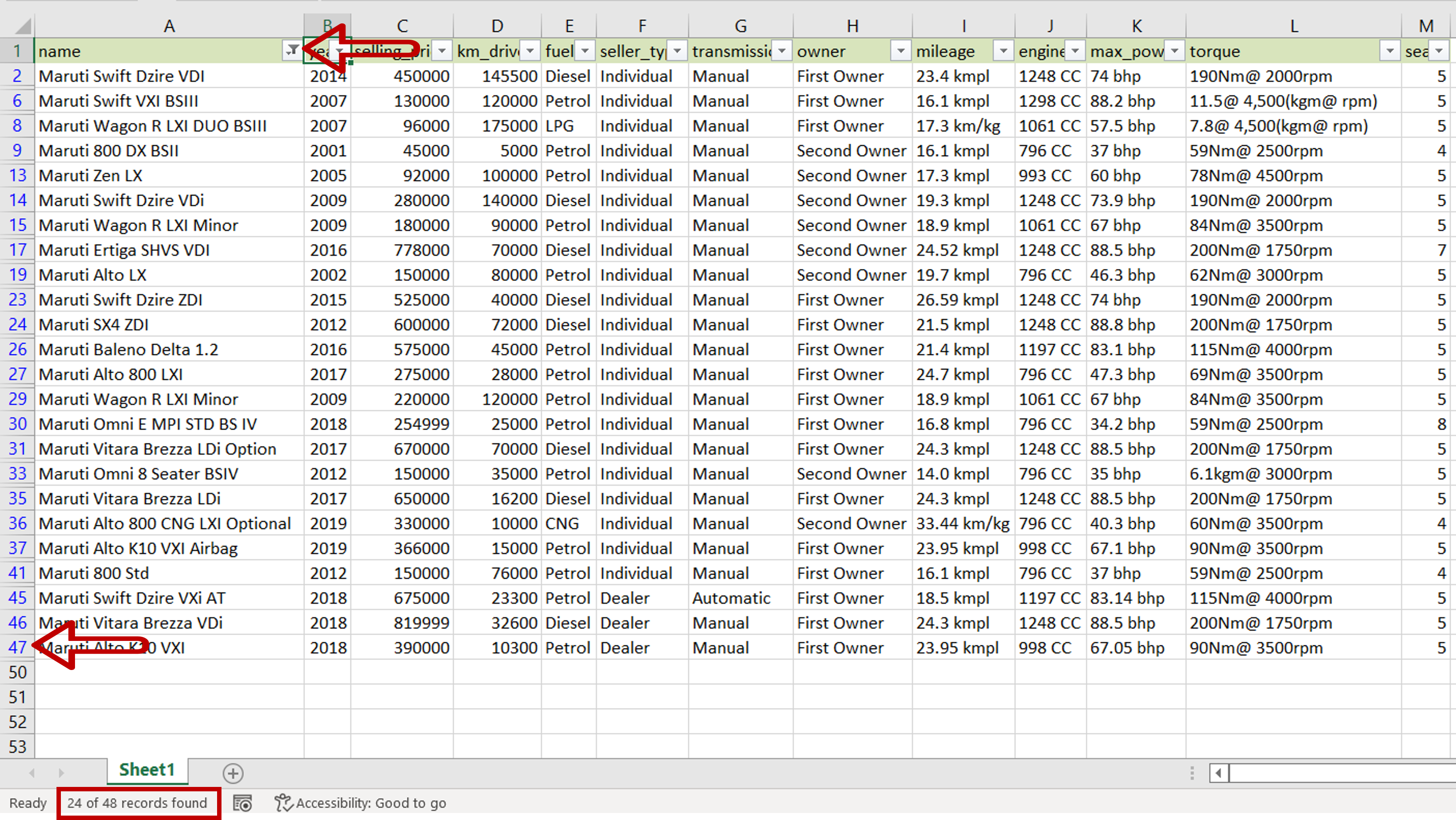
– Only those rows that have ‘Maruti’ in the ‘name’ column are displayed
– A filter symbol appears on the in-column filter in the ‘name’ column to indicate that a filter has been applied
– The row numbers of the filtered rows appear in blue font to indicate that they are part of the filter results
– The number of records returned based on the filter condition is displayed in the status bar
Step 4 – Apply the second condition
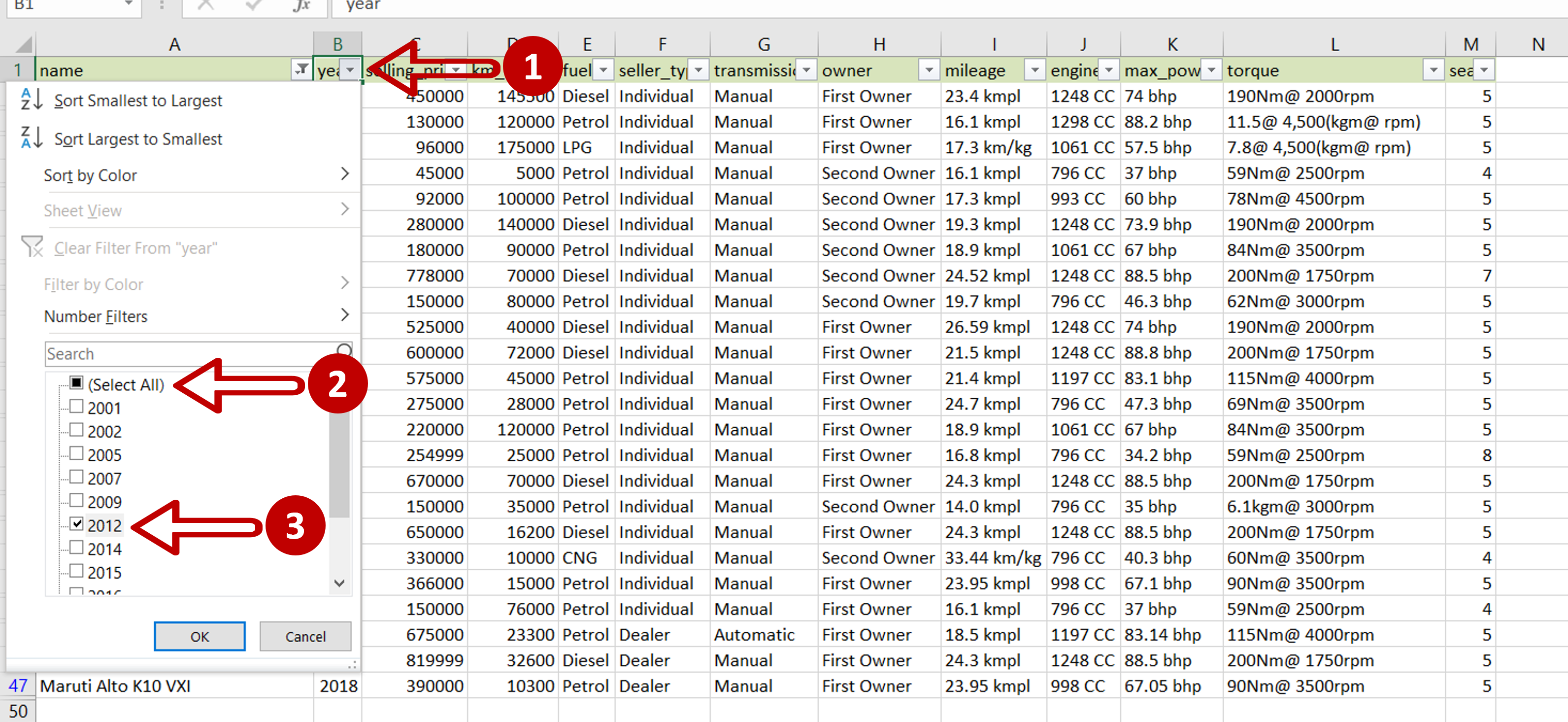
– Click the filter button in the ‘year’ column
– Uncheck Select All
– Select ‘2012’
– Click OK
Step 5 – Check the final list
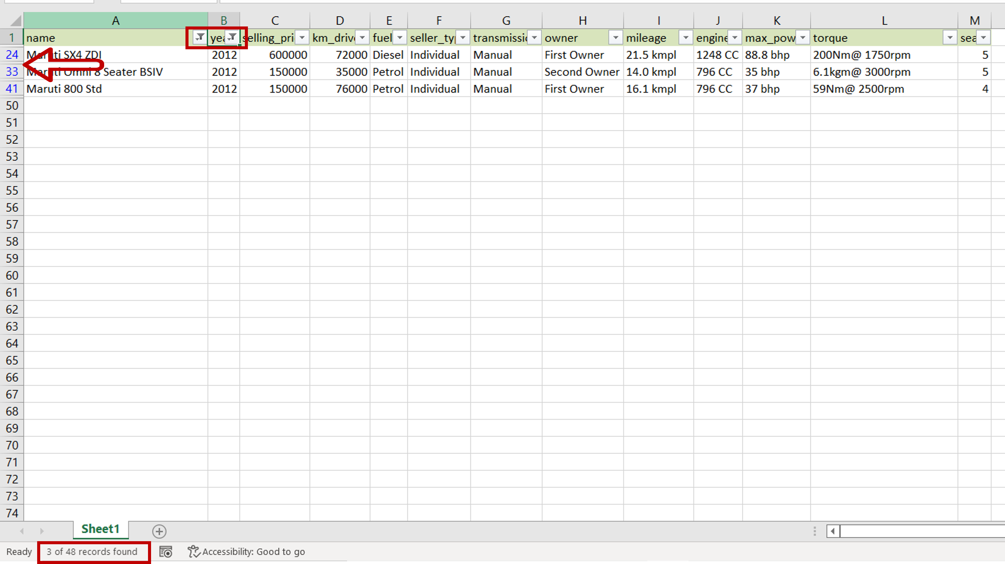
– Only those rows that have ‘Maruti’ in the ‘name’ column and ‘2012’ in the ‘year’ column are displayed
– A filter symbol appears on the in-column filter in the ‘name’ and ‘year’ columns to indicate that filters have been applied to these columns
– The row numbers of the filtered rows appear in blue font to indicate that they are part of the filter results
– The number of records returned based on the filter conditions is displayed in the status bar
Step 6 – Copy the data
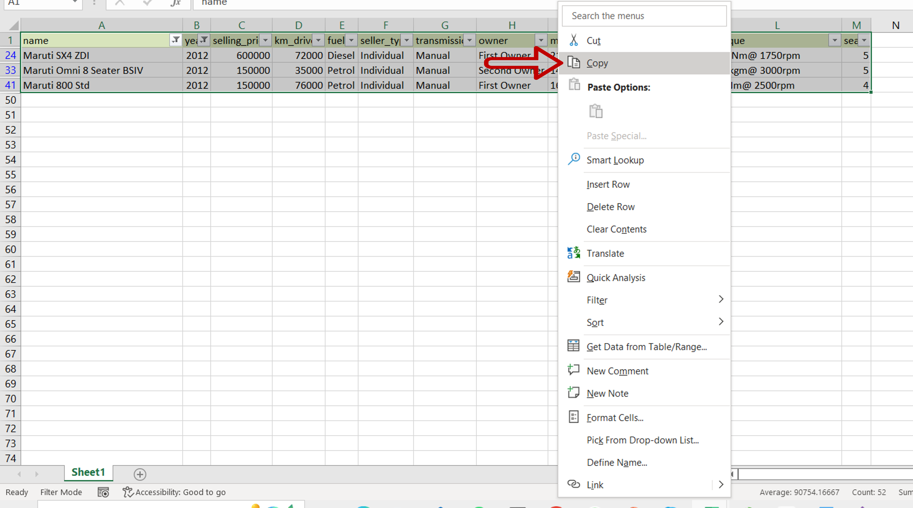
– Select the filtered data
– Right-click and select Copy from the context menu or press Ctrl+C
Step 7 – Paste the data
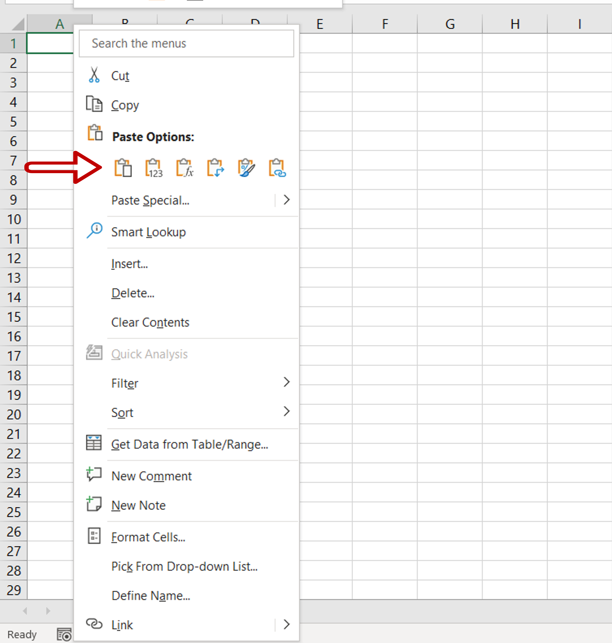
– Go to a new sheet
– Select cell A1
– Right-click and select Paste from the context menu or press Ctrl+V
Step 8 – Check the result
– Maruti cars from the year 2012 have been extracted from the dataset


