How to edit an array in Excel

Excel is a powerful tool for managing data and analyzing large amounts of information. One of the most useful features of Excel is the potential to work with arrays. Arrays are a group of related values that are organized in rows and columns. They can be used for a variety of tasks, such as performing calculations, creating charts and graphs, and filtering data.

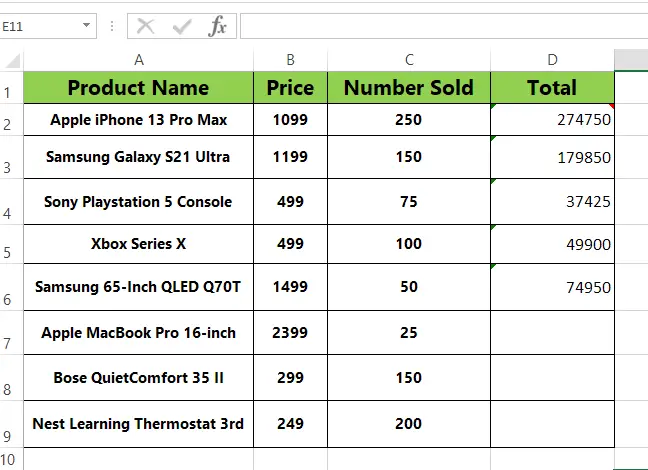
In this tutorial, we will understand how to edit an array in Excel using different methods. Here we have an example dataset that consists of Product name, Price, Number Sold and Total. Follow the simple steps given below to edit an array in Excel. Let’s examine the dataset first.

Method – 1  Extending Multi-cell Array formula.

Step – 1 Select the cells.

• Click on the first cell in the Total column.
• Look at the formula bar to see the array formula that is being used.
• Select all the cells including the cells where you want to extend your formula

Step – 2 Change the formula.

• Change the formula in the formula bar according to your need.
• Then press Ctrl + Shift + Enter this indicated to Excel that the array formula is being used.

Method – 2 Single-cell Array formula

Step – 1 Select a cell.

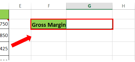
• To show how the Single-Cell array formula works we will be finding the Gross Margin of all the sales.
• For this select the cell where you want to show the Gross Margin.

Step – 2 Type the formula.

• In the selected cell type the formula for the array.
• Here we are finding Gross Margin so the formula will be

SUM(C2:C9*D2:D9)

• After typing the formula press Ctrl + Shift + Enter this will indicate to Excel that the array formula is being used.

Method – 3 Taking Transpose of Array.

Step – 1 Select the cells.

• Select the empty cells according to your data.
• In our case we selected 4 rows and 9 columns to display the transpose of the data as shown below.

Step – 2 Apply the Formula.

• Click on the formula bar after selecting the cells.
• Type the formula.
• Syntax of the formula is:

=TRANSPOSE(Range of the cells)

• In our case formula will be:

=TRANSPOSE($A$1:$D$6)

• After typing in the formula press Ctrl + Shift + Enter to indicate it as an array.