How to drill down in Excel

You can watch a video tutorial here.

When you have a large amount of data that runs into many rows and columns, you can group either the columns or rows so that the data becomes more manageable. The groups can be made by collapsing rows so that you can then drill down to the more detailed data. This is useful when you have subtotals within the sheet and would like to group the cells so that only the subtotals are displayed. The method shown below is for rows and can be used for columns as well.

Option 1 – Group the rows individually

Step 1 – Select the rows

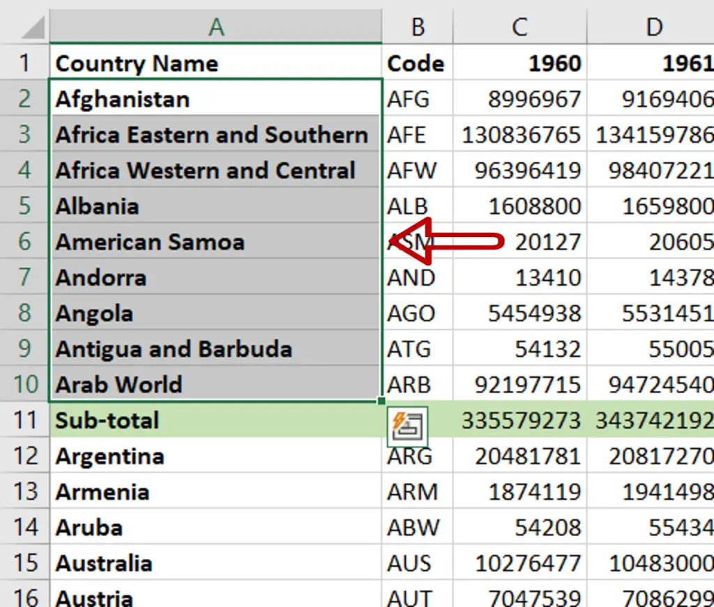
• Select the rows to be grouped

Step 2 – Open the Group box

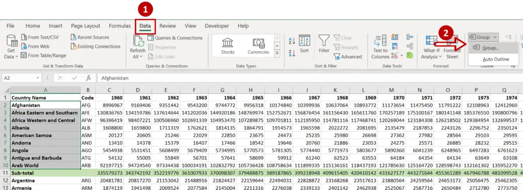
• Go to Data > Outline
• Select Group from the Group dropdown

Step 3 – Choose the cells to group

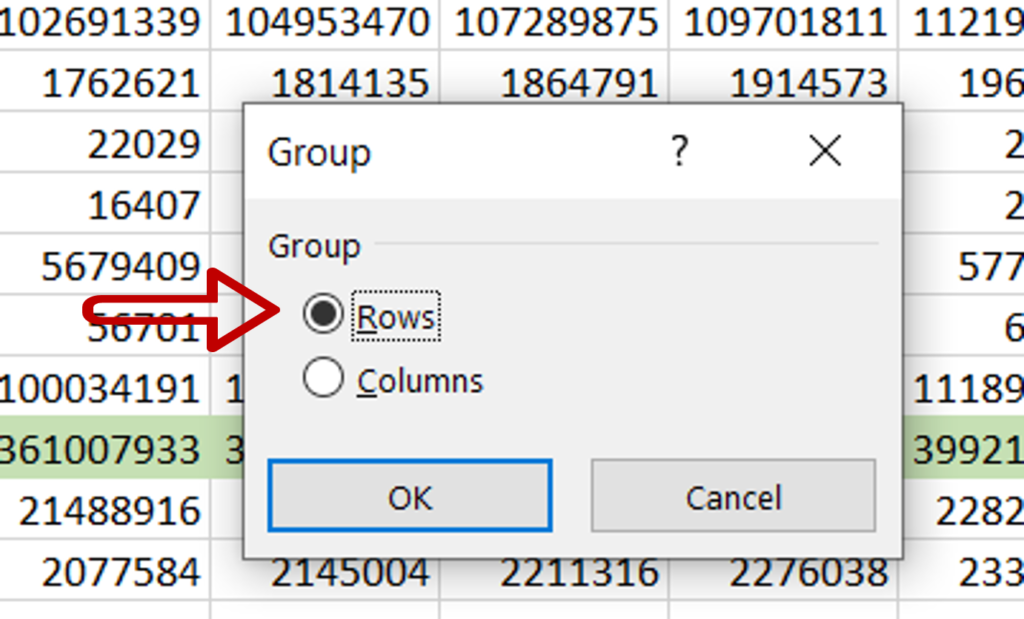
• In the pop-up, select Rows
• Click OK

Step 4 – Collapse the rows

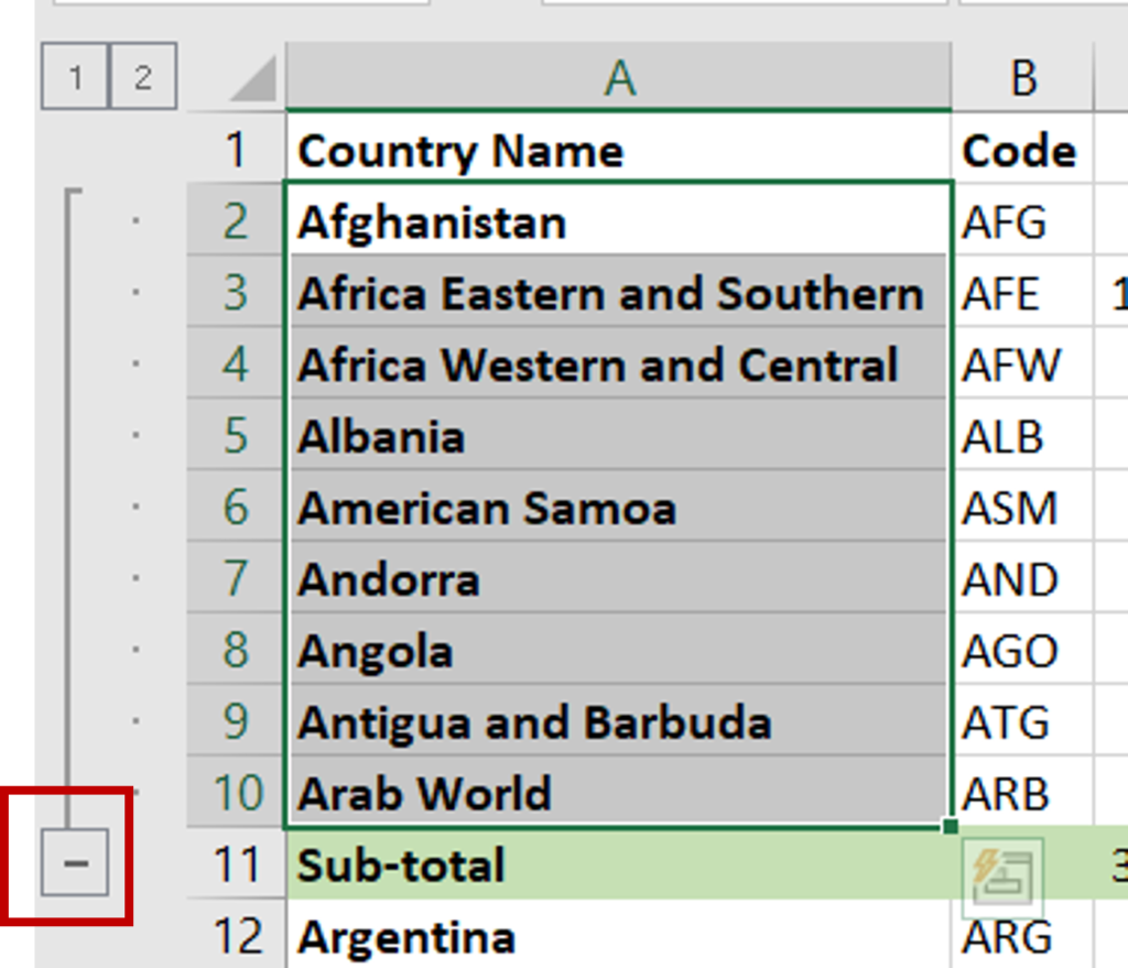
• Click on the minus sign (-) shown at the bottom of the group indicator

Step 5 – Check the result

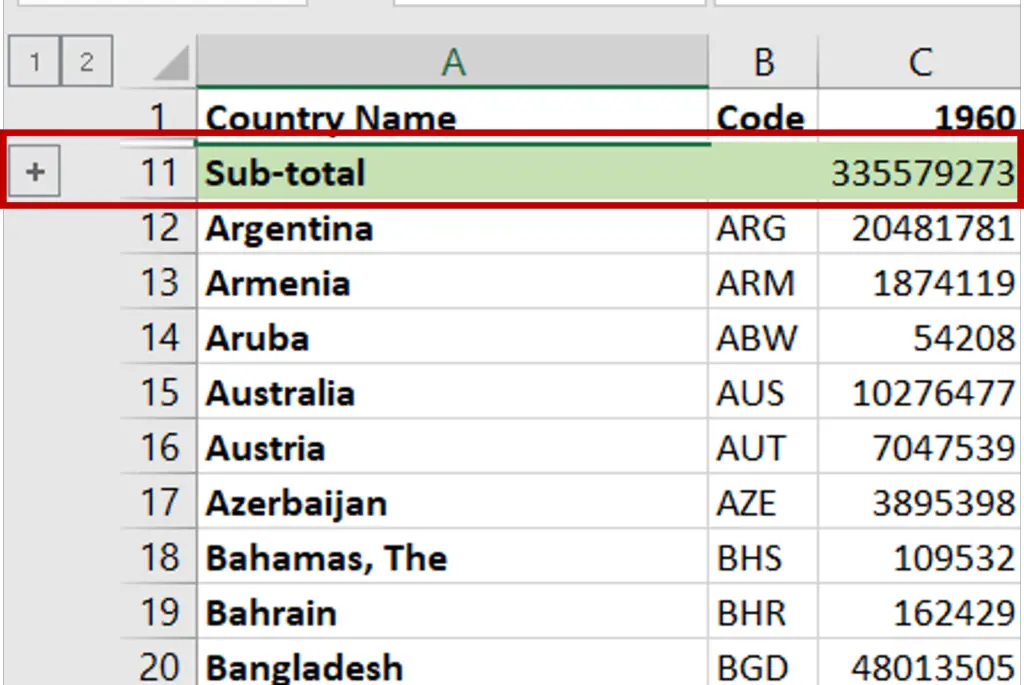
• The selected cells will be collapsed
• Click on the plus sign (+) to drill down

Step 6 – Create more sections

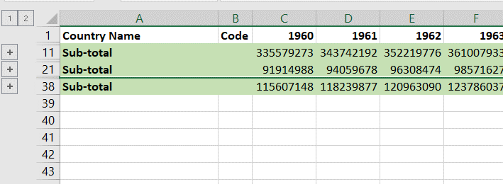
• Repeat Steps 1 to 5 to collapse more rows
• From the grouped view you can drill down to get more details

Option 2 – Use Auto Outline

Step 1 – Select the entire sheet

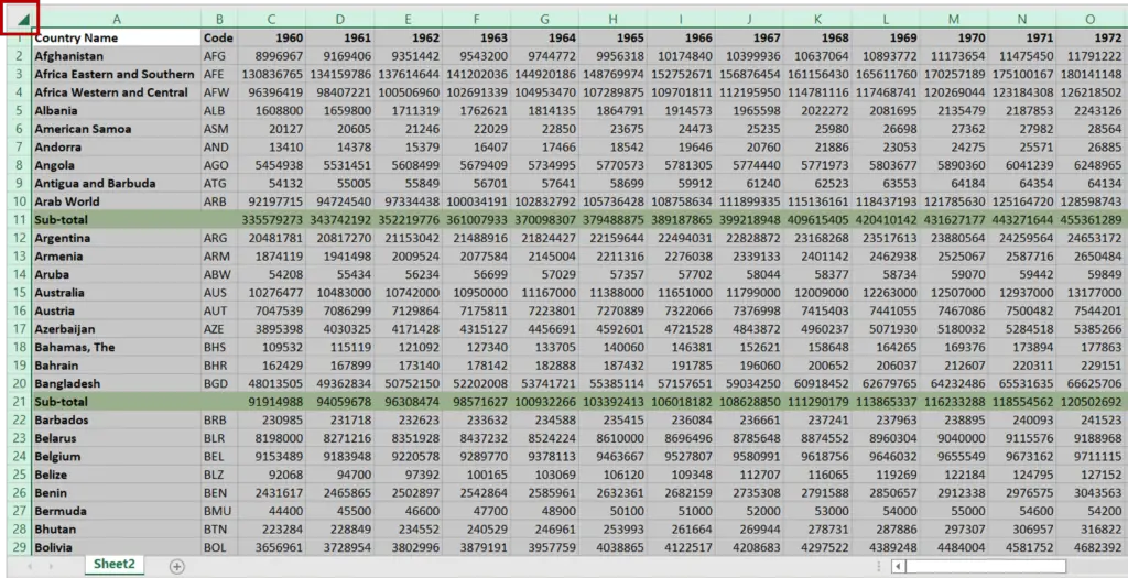
• Select the entire sheet by clicking in the top left corner

Step 2 – Choose Auto Outline

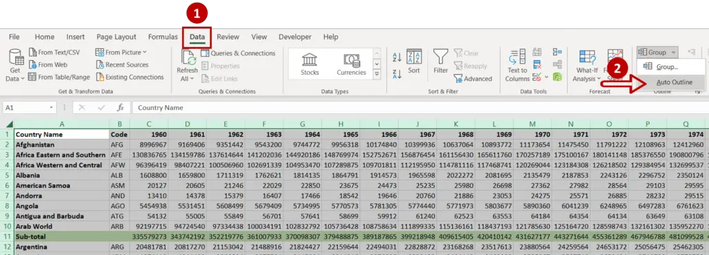
• Go to Data > Outline
• Expand the Group menu
• Choose Auto Outline

Step 3 – Group the rows

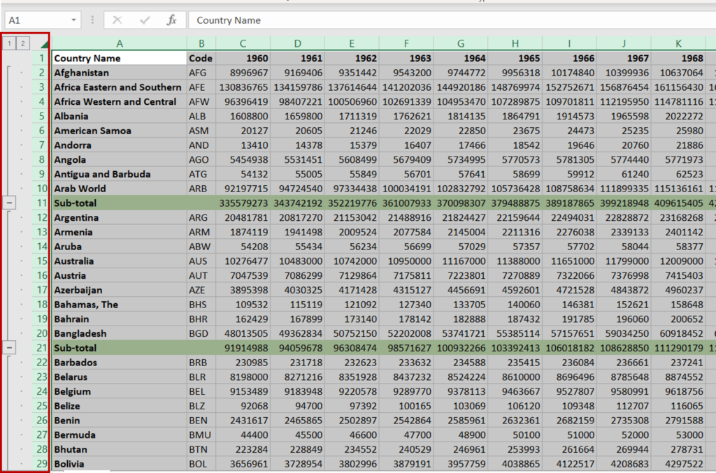
• The entire sheet is grouped according to the ‘Sub-total’ rows
• Click on the number 1 to group the rows

Note: This feature will work only if there are discernible sections in the data – in this case, the sub-totals

Step 4 – Check the result

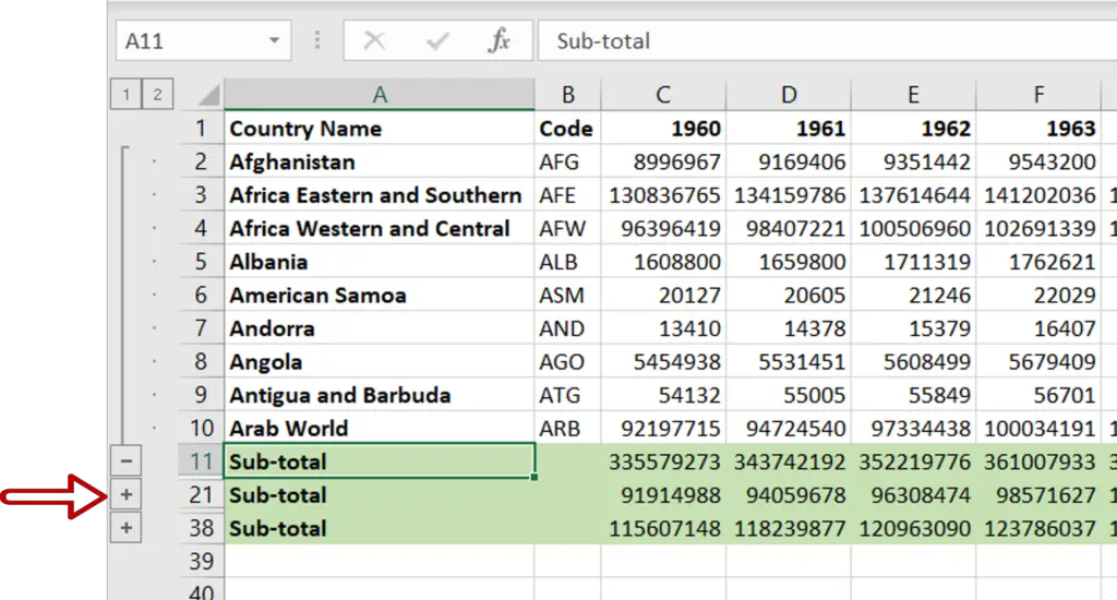
• Click on the plus sign (+) to drill down any of the grouped sections