
How to do Conditional Formatting with Multiple Conditions in Excel
 By
SpreadCheaters
By
SpreadCheaters
In this tutorial we have a dataset which contains 9 student names and their marks out of 100, we will be performing Multiple Conditional Formatting on this dataset.
Conditional formatting is a powerful feature in Microsoft Excel that enables users to format cells automatically based on certain criteria or conditions. It is a great tool for making your data more readable, visually appealing, and easier to analyze. With conditional formatting, you can highlight cells that meet specific criteria, such as values that are above or below a certain number, cells that contain certain text or values, or cells that are duplicates. You can also create rules based on formulas or use pre-built rules to format cells, such as data bars, color scales, and icon sets.
Step 1 – Open Conditional Formatting
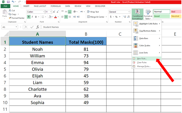
– Select the data on which you want to do Conditional Formatting.
– In the Styles group click on Conditional Formatting a drop down menu will appear.
– Click on New Rules.
Step 2 – Define the Rule
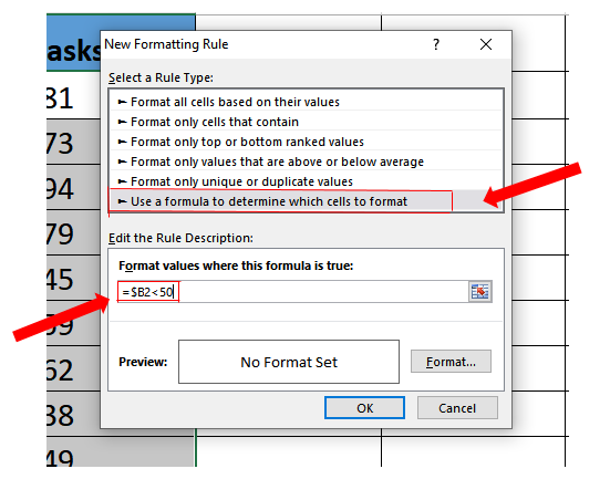
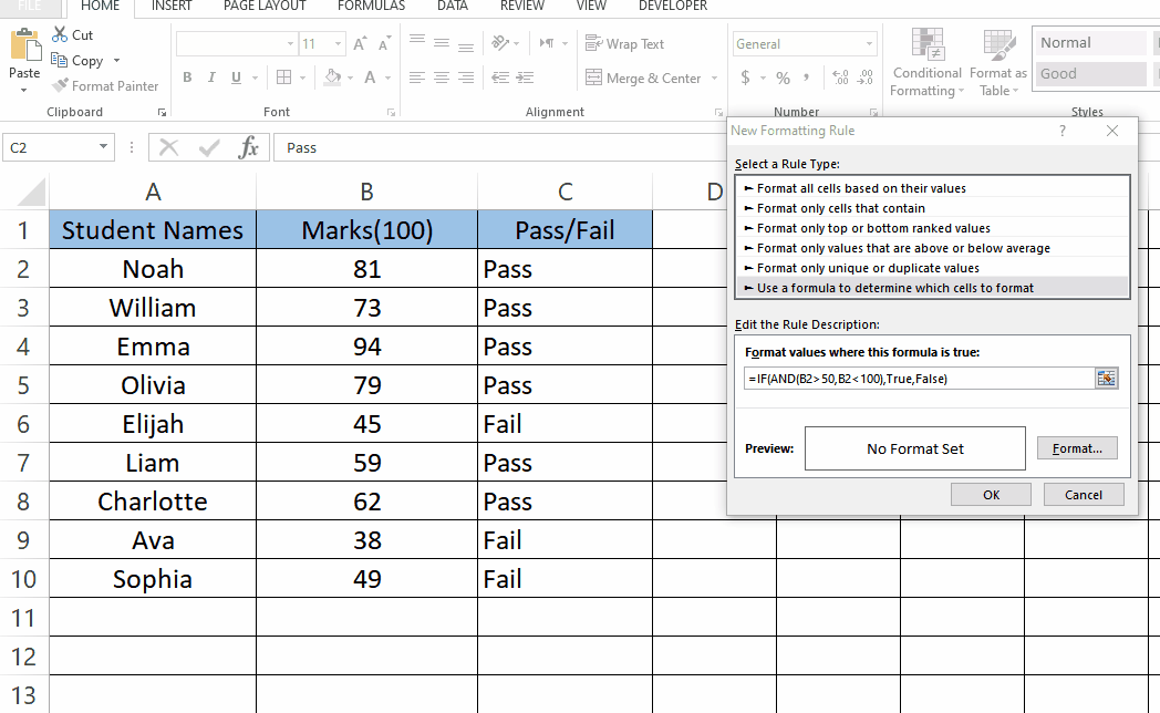
– After opening new rules click on “Use a formula to determine which cell to format”.
– Now type in the formula.
Step 3 – Multiple Formatting with two formulas.
– For Formatting we have used two different formulas which are given below
=$B2<50 (To highlight the students with marks less than 50 in Red)
=$B2>50 (To highlight the students with marks less than 50 in Green)
– To highlight the data click on format after typing in the formula.
– Choose the color you want to highlight the data with (Green & Red).
Step 4 – Multiple Conditional Formatting

– We can also use multiple conditions for conditional formatting. For example, if we wish to implement a condition to turn only those students’ marks to green where they have achieved more than 50 and less than 100 marks then we can combine both conditions using the following formula.
=IF(AND(B2>50,B2<100),True,False)
– AND contains two condition, both the condition needs to be true In AND statement to continue
– IF statement is used which will apply the format if the AND condition is True otherwise it will be considered as False and the format will not be applied.
– If both the conditions(IF,AND) are True Green color will be applied to the marks greater than 50.


