
How to do a SUMIF in Excel
 By
SpreadCheaters
By
SpreadCheaters
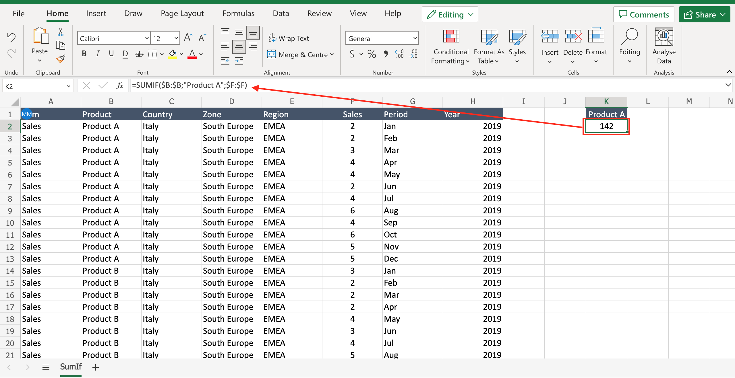
Let’s assume you have a table with the sales for different products and you want to know how many items of a certain product have been sold. To do that you have to know how to perform a sumif in Excel, a function that allows to sum only certain values decided by the user. To do so proceed as follows.
Step 1 – Select the cell where to insert the function
– Select the cell by clicking on it or with the keyboard arrows.
Step 2 – Write the function
– Inside the selected cell write “=” to let the tool understand you want to insert a function;
– Start writing “SUMIF” and the tool will suggest the SUMIF function;
– Select the range where you have the list of items that the function will filter. In the example the range is the column where there are the product names, because the goal is to sum only one product name. Press “F4” to block the cells, in this way you can copy the formula down the column avoiding to move the range.
– Select the criteria the function will follow to filter only the data you want to sum. In the example we want to sum only “Product A” sales so the criteria will be “Product A”.
– Select the sum range, so the range where you have the numbers to sum once the criteria matches. – In the example the range is the column where the sales of each product are stored.
– Close the parenthesis;
– Press enter to confirm the function.


