How to create sentence case in Excel

Microsoft Excel is a computational software tool which has many versatile tools for mathematical calculations. However, it doesn’t have many useful tools when it comes to text editing in Excel. One of the most common problems is that Excel doesn’t provide any direct tool for changing the case of text to proper sentence case. 

In this tutorial we’ll learn the methods to convert the case of text to sentence case. There are two methods that can be used for this purpose;

• Use Flash Fill tool i.e., CTRL+E
• Use a combination of formulas

Method 1 – Use Flash Fill to change case

Step 1 – Create one or two sample data points and use CTRL+E

• To change the case of text to sentence case using Flash Fill (CTRL+E) we will need to create one or two data points to train Excel’s AI engine. 
• Then simply press CTRL+E and the rest of the work will be done by Excel as shown below;

Method 2 – Use a combination of formulas

Step 1 – Create the appropriate formula

• To change the case of the text to sentence using a combination of formulas, we need to create an appropriate formula which is as follows;

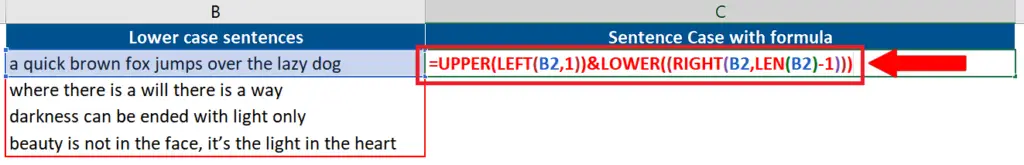
We used the following formula, which is lengthy but not complex. There are two parts of the formula and both are separated by different colors. Let’s understand the formula part by part.

=UPPER(LEFT(B2,1))&LOWER((RIGHT(B2,LEN(B2)-1)))

UPPER(LEFT(B2,1))

The left part of the formula first uses LEFT(B2,1) which grabs 1 character from the left of the text present in B2. The output of this function will be the character “a”. Then we passed this output to UPPER function which changed the case of character “a” to “A”.

LOWER((RIGHT(B2,LEN(B2)-1)))

The inside function of this right half is RIGHT(B2, LEN(B2)-1)

RIGHT returns the last character or characters in a text string, based on the number of characters you specify in the second parameter. The output of this function in our case will be all characters of the text string present in B2 except the first character because we passed a number in the second parameter of RIGHT function which is 1 less than the total length of the text in B2. Then we passed this output to LOWER function which converts the text case to lower case. 

&

The ampersand character joins the outputs of the functions written left and right of this operator and we get our desired output which is 

A quick brown fox jumps over the lazy dog

Step 2 – Implement the formula

• Now that we have created a working formula, it’s time to implement it and get the desired results. So, write the formula in the appropriate cell and press enter. You will get the desired output. Now double click the fill handle to implement the formula to the rest of the data.