
How to create progress bars in Excel
 By
SpreadCheaters
By
SpreadCheaters
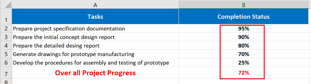
Let’s consider this dataset which has the information about the progress of various tasks in a design project and then overall project status is calculated by taking the average of progress of all tasks. Let’s learn how to create progress bars in Excel by using conditional formatting following the steps mentioned below.

Excel is a very powerful tool to perform mathematical and statistical calculations on numeric data. However, it provides a variety of tools and functions to visualize the data quantitatively as well. If you are a project manager then you must have created Project Schedules and Task Status in Excel. It is very handy to create and use progress bars to keep track of the status of the tasks and overall project status as well.
Step 1 – Select quantitative data only

– Progress bars are a data visualization tool; however, it requires quantitative data to work. Therefore, select only the quantitative data in your dataset, which in our case are the cells from B2:B7.
Step 2 – Locate Data Bars from Conditional Formatting options
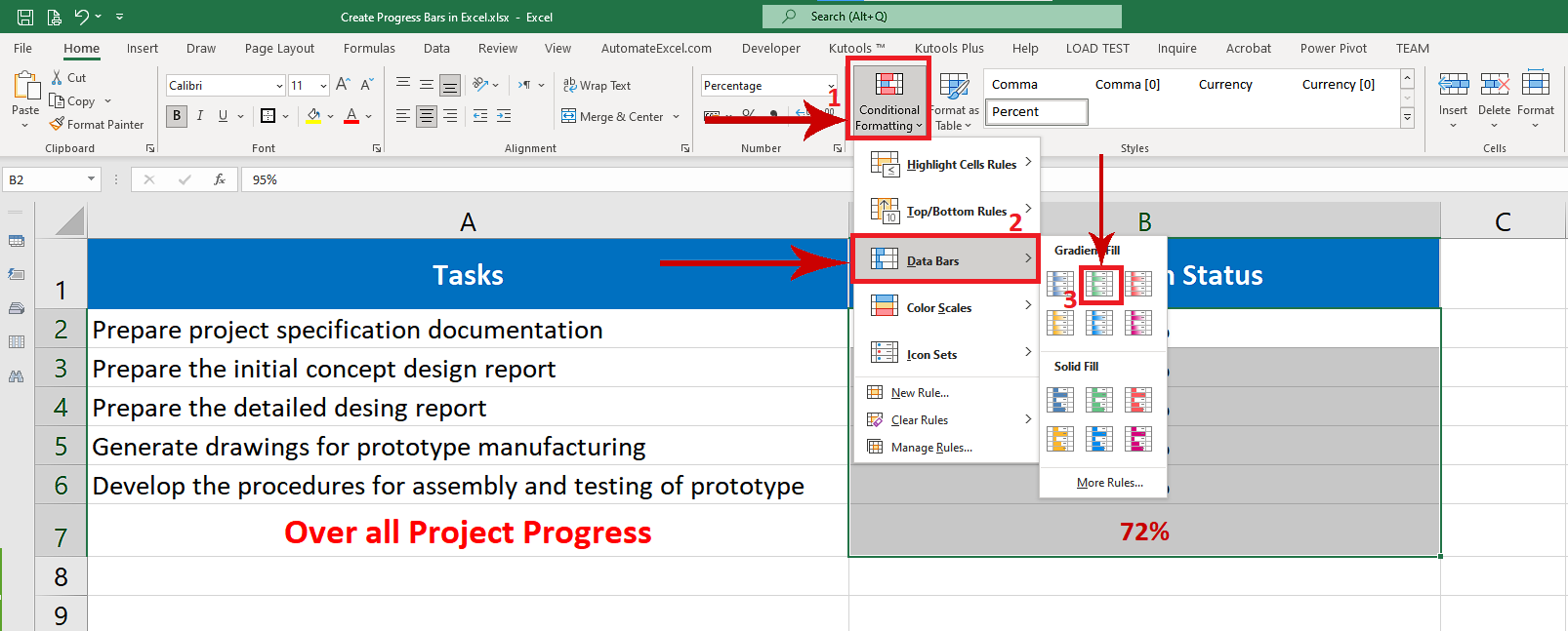
– In the HOME tab, locate the Styles group and click on the Conditional Formatting dropdown arrow.
– Now go to Data Bars options and any one option out of Gradient Fill or Solid Fill. For this tutorial we’ll choose Gradient Fill.
Step 3 – Apply Progress bars to visualize the data
– After selecting the quantitative data, when you click on the Gradient Fill in the last step, it will automatically apply the conditional formatting and you will see the Progress Bars along with data as shown above. The good thing about these is that these are dynamic bars so the length of the progress bar will change accordingly on the go.


