How To Create Lookup Table In Excel

You can watch a video tutorial here.

A lookup table contains a master list of values that are usually associated with a key. The key is used to ‘lookup’ the value. Lookup tables can be used to help you quickly find data from a large dataset. Suppose you have a list of 500 students and you need to frequently use the student ID to find the name of the student. You can use the IDs and the names to build a lookup table and then use the table whenever you need to find the name of a student.

In Excel, the table is created using the key-value pairs and then we can use the VLOOKUP() function to use the lookup table.
1. VLOOKUP() function: this searches for a value in the left-most column of a range, and returns the value in the column specified from the row of the match in the range.
*Syntax: VLOOKUP(lookup_value, table_array, col_index_num, range_lookup)
i. lookup_value: the cell reference of the first value in the key column from Table 1 (Name)
ii. table_array: the range of Table 2 which is made constant with the addition of dollar signs ($)
iii. col_index_num: the number of the column in Table 2 that has to be retrieved (1 i.e. the Name)
iv. range_lookup: TRUE will return an approximate match, FALSE will return an exact match

2. A few things to keep in mind when using Vlookup:
*The key must always be in the left-most column of the table being referenced
*The table that is being referred to must always be sorted on the key, in ascending order
*It is better that the key being used has unique values or else the function may not return the desired result

Step 1 – Create the table

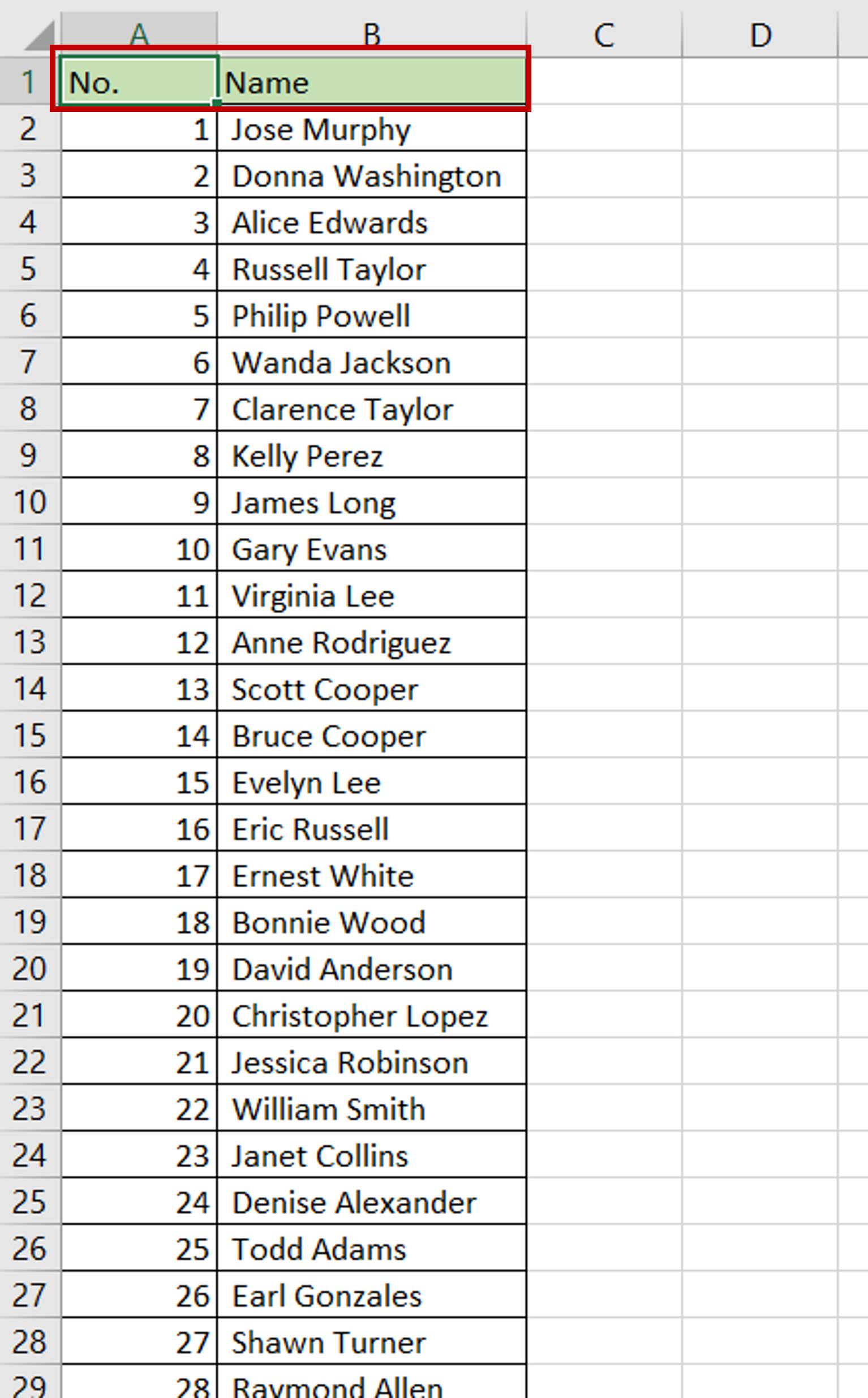
– Create a column for the key i.e. ‘ID’
– The column should have unique values
– Add the values i.e. ‘Name’

Step 2 – Add fields for looking up

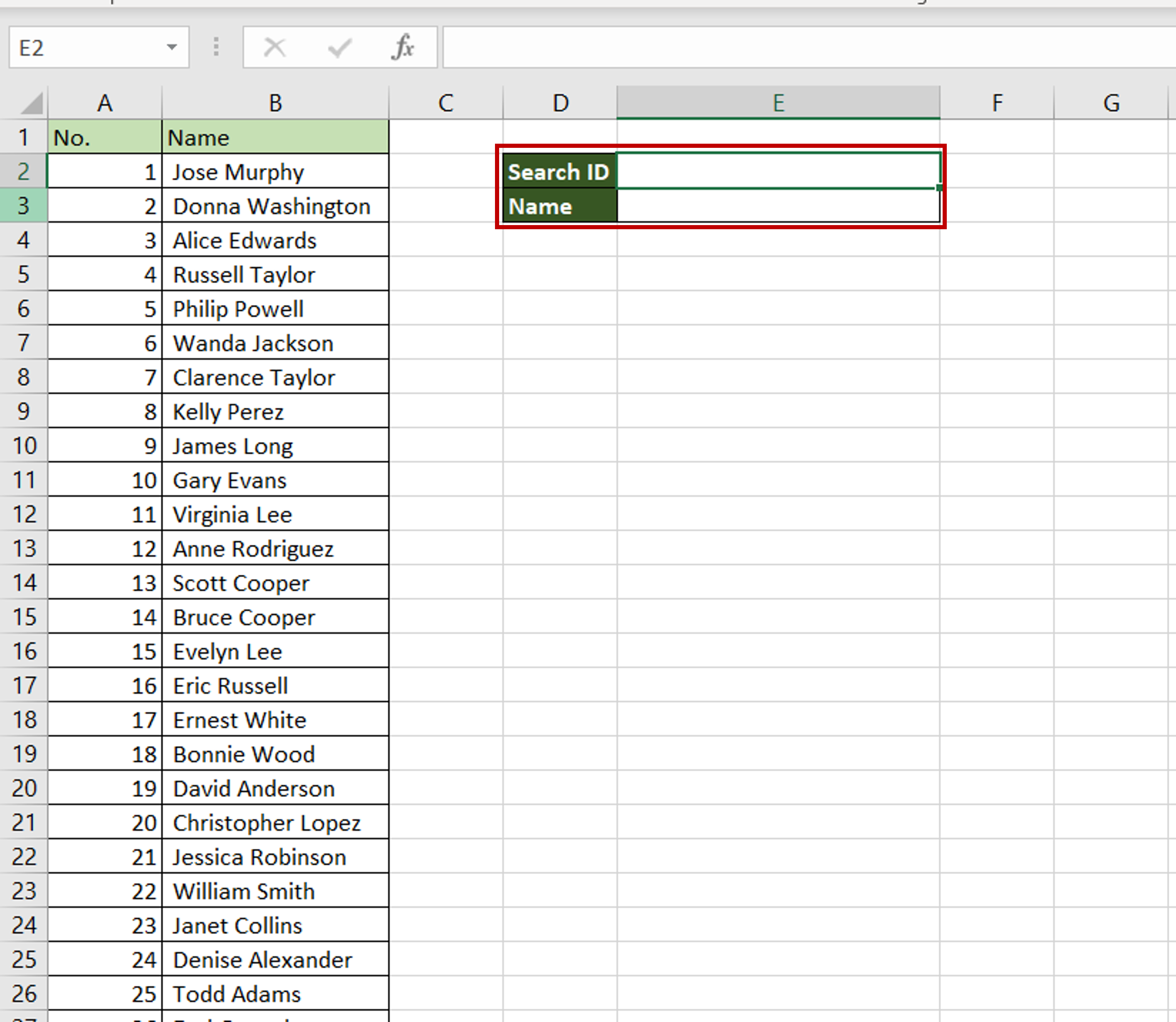
– Add a field for entering the key i.e. the ‘ID’ to be used for the search
– Add another field for displaying the result

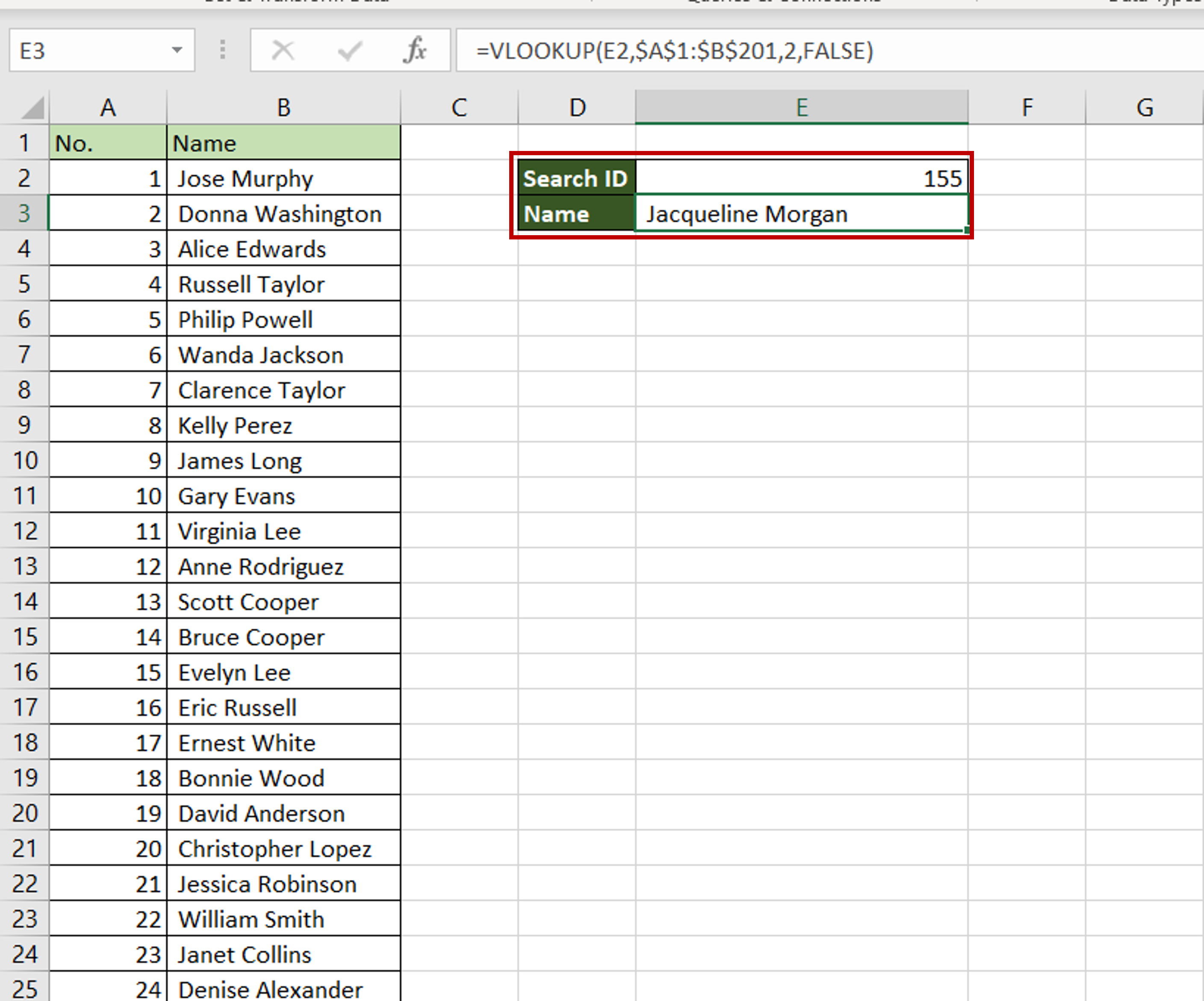
Step 3 – Create the formula

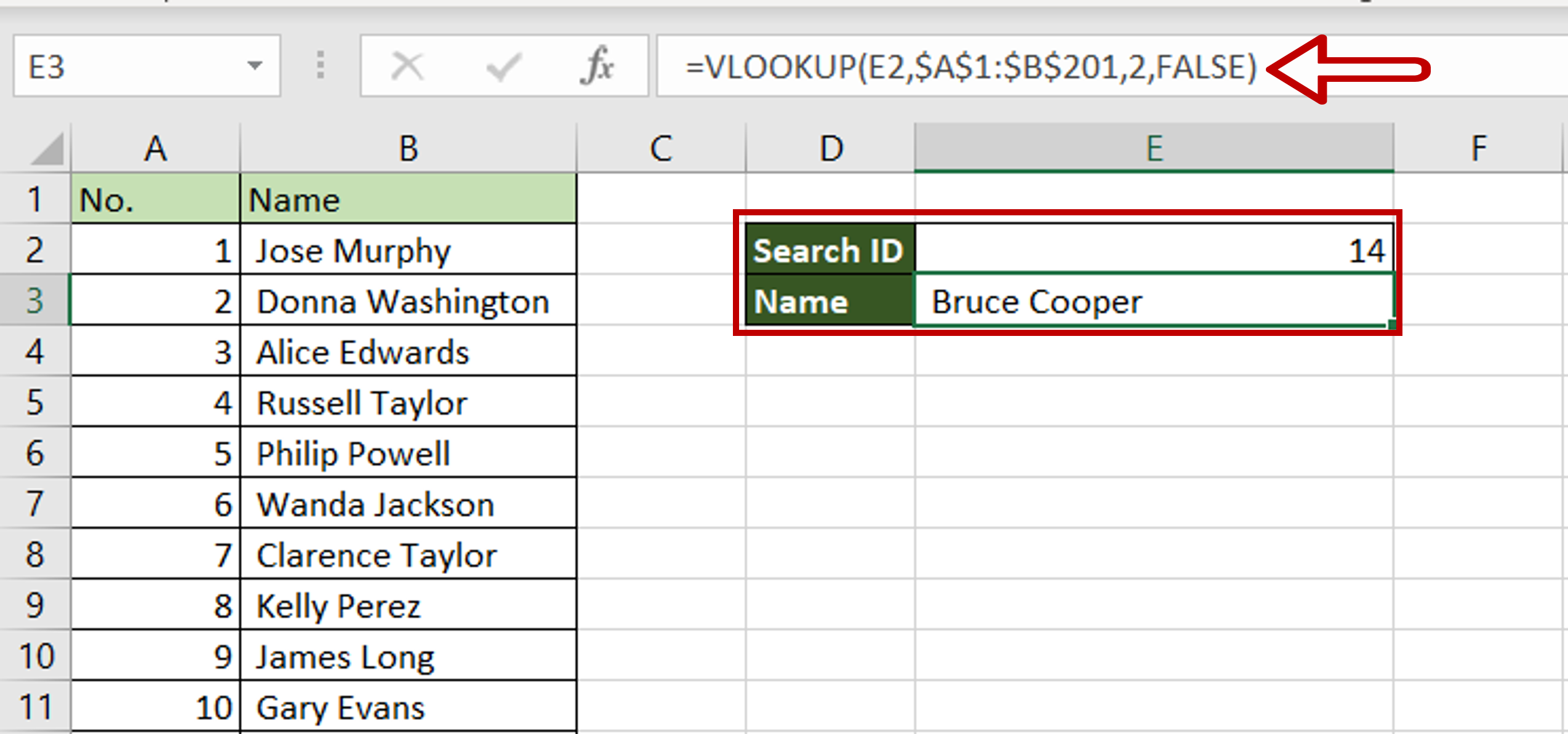
– Enter any number in the field for ‘Search ID’
– Select the cell where the result is to be displayed
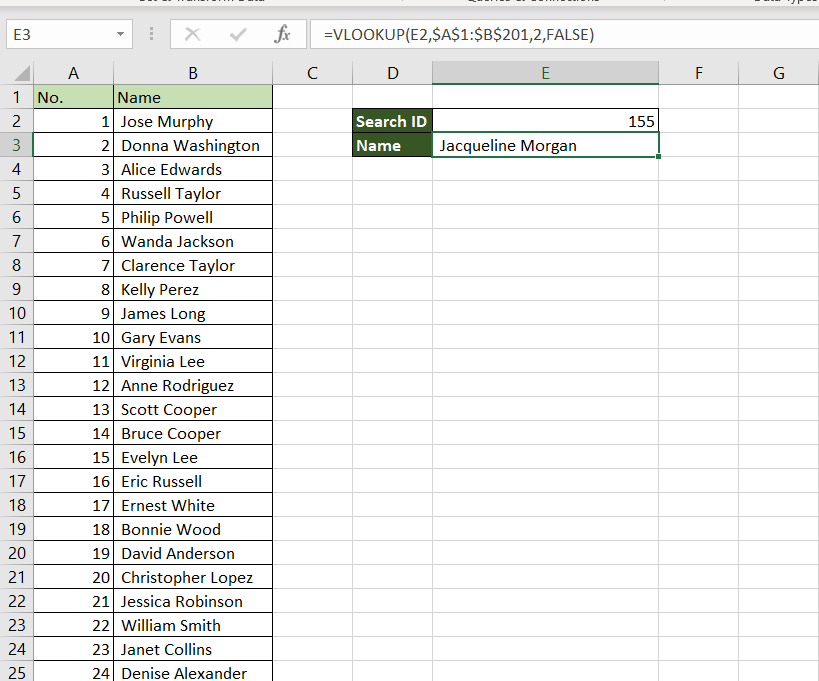
– Type the formula using cell references:
=VLOOKUP(Search ID, $range of the table$,2,FALSE)
– The range of the table is made constant by selecting the cell reference and pressing F4
– Press Enter