
How to create an organizational chart in Excel from a list
 By
SpreadCheaters
By
SpreadCheaters
You can watch a video tutorial here.
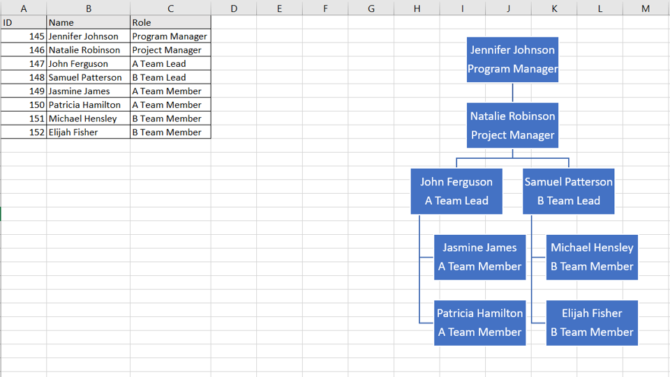
Several tools are common across Microsoft Office applications and the SmartArt suite is one of them. You may need to create a hierarchy when you are working in Excel. For example, if you are preparing a report related to Human Resources, you may want to include a chart depicting the team structure. In Excel, this can be done using the ‘Hierarchy’ graphic from the SmartArt suite of tools.
Step 1 – Open the Choose a SmartArt graphic dialog box
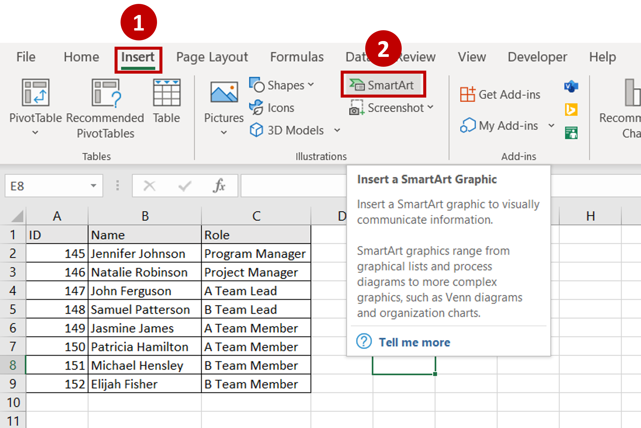
– Go to Insert > Illustrations
– Click the SmartArt button
Step 2 – Select a hierarchy
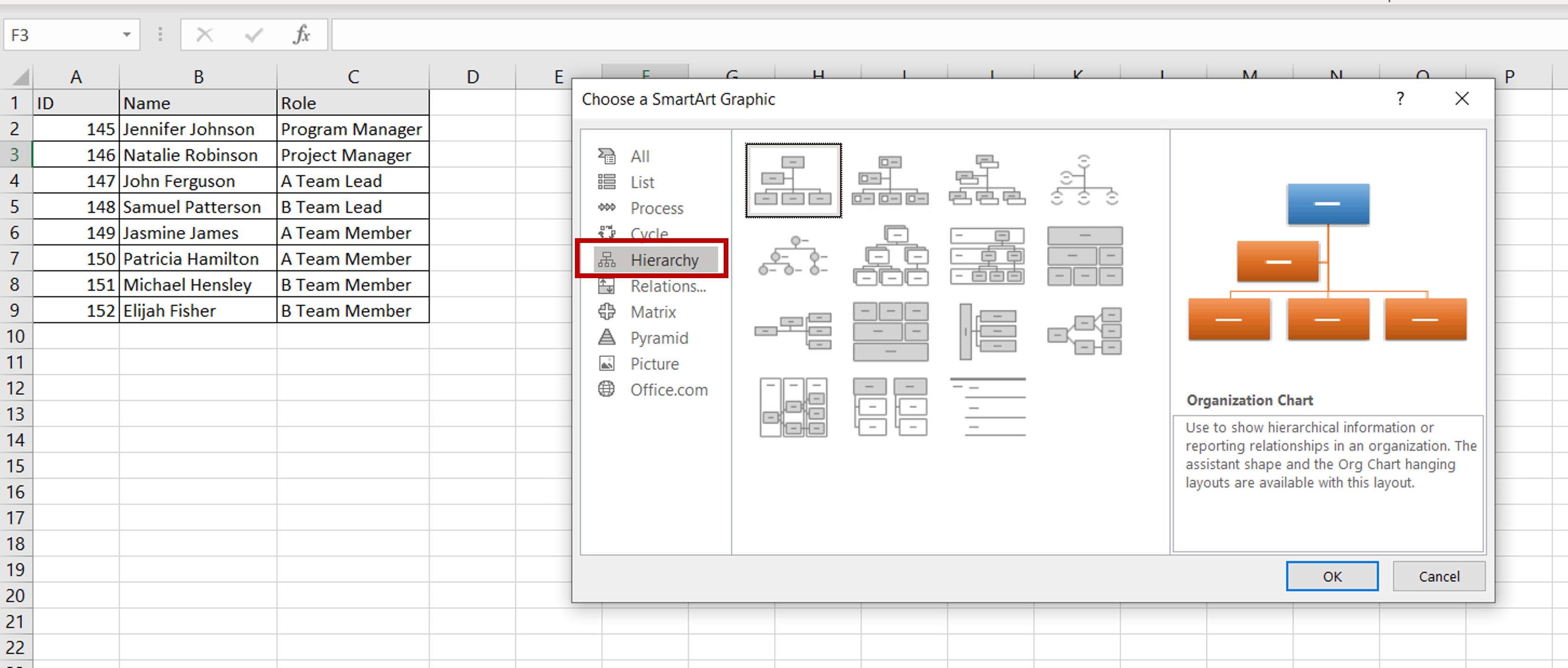
– Go to Hierarchy
– Pick any one of the options displayed
– Click OK
Step 3 – Copy the data
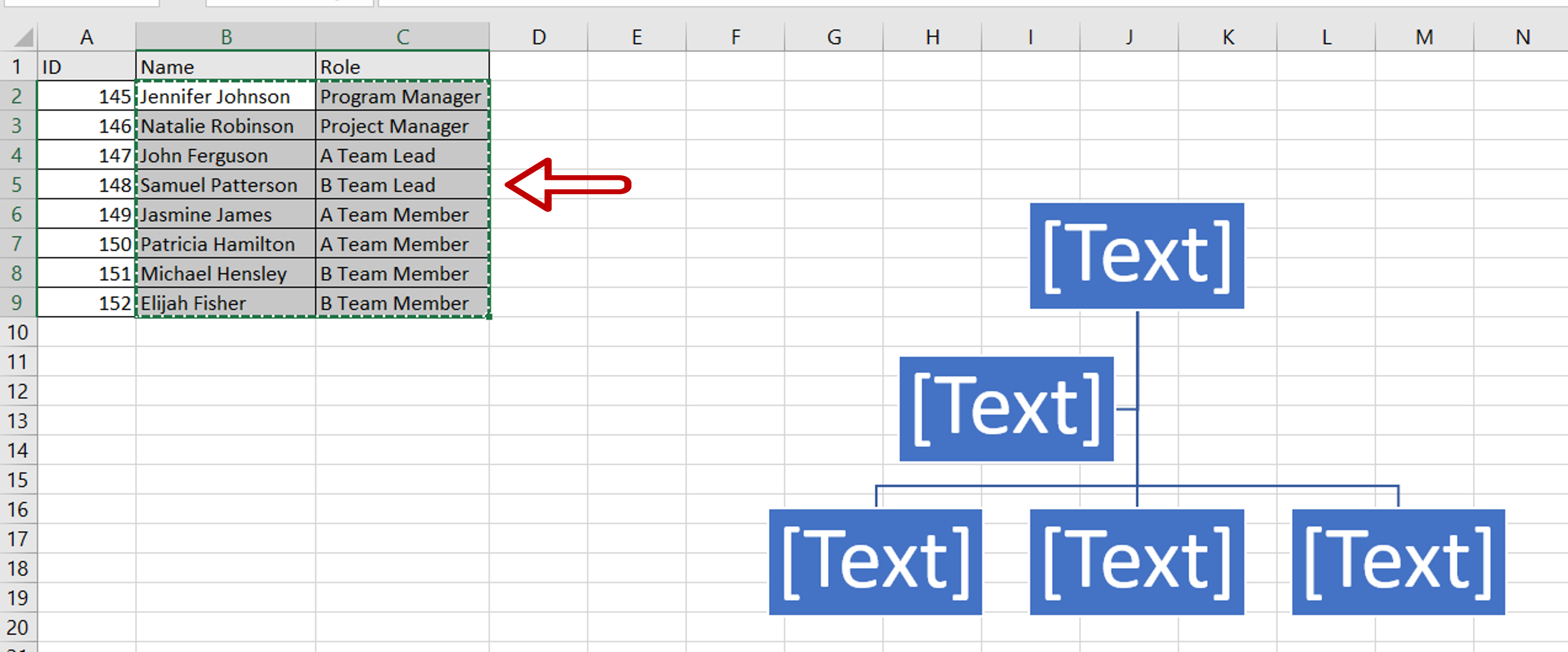
– Select the ‘Name’ and ‘Role’ columns and press Ctrl+C
Step 4 – Open the text pane
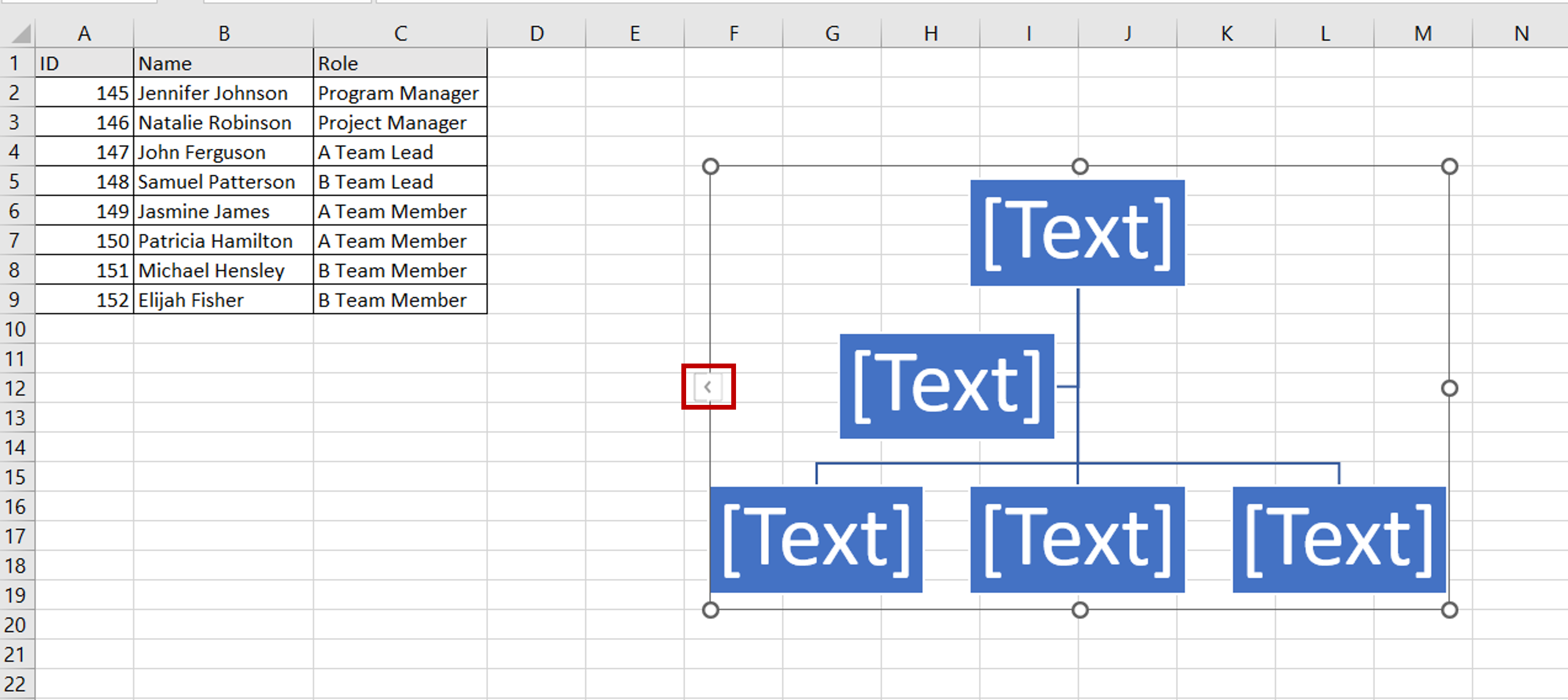
– In the chart that is inserted into the worksheet, click on the arrow on the left border
– This opens the text pane
Step 5 – Paste the names
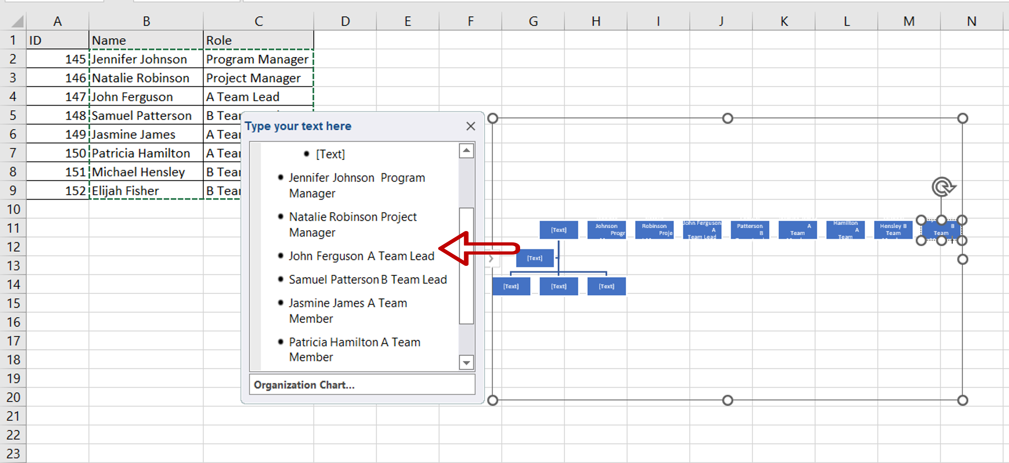
– Place the cursor in the text pane
– Press Ctrl+V
– The names and roles are pasted into the text pane
– The chart shows the name and roles at the same level
Step 6 – Create the hierarchy
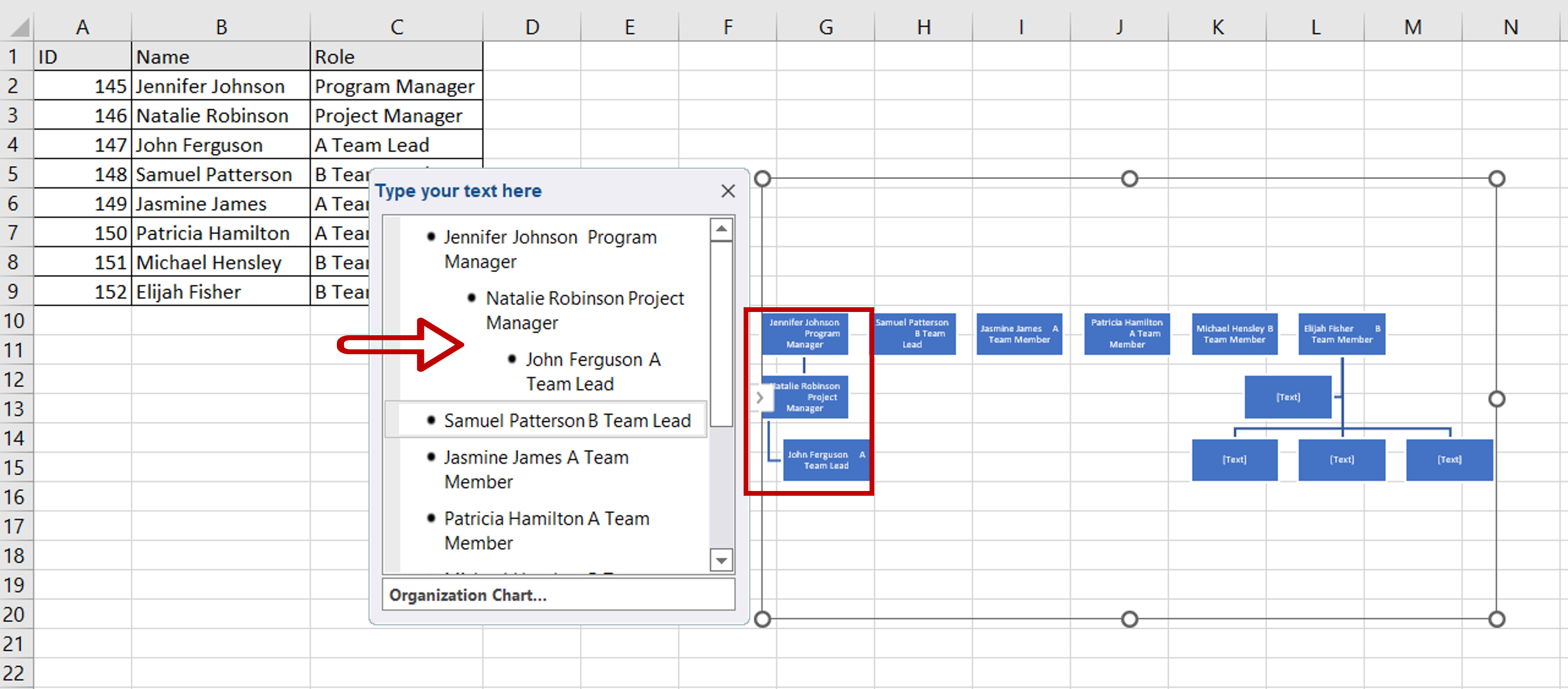
– Place the cursor in front of the Project Manager’s name in the text pane
– Press TAB once to indent to the first level of the hierarchy
– Place the cursor in front of the Team Leader’s name in the text pane
– Press TAB twice to indent to the second level of the hierarchy
– The chart is updated based on the movements
Step 7 – Move the team members
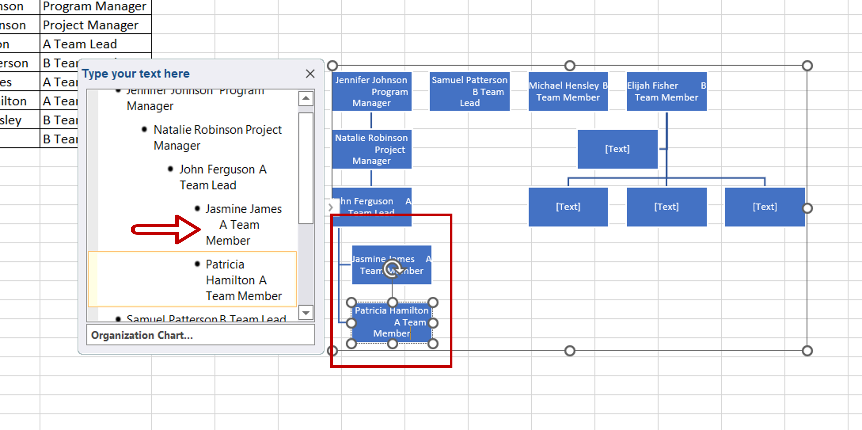
– Select the A team members
– Press Ctrl+X
– Place the cursor at the end of the A Team Lead’s name
– Press Enter
– Press TAB
– Press Ctrl+V to paste the team member’s names
– The chart is updated accordingly
Step 8 – Finish the chart
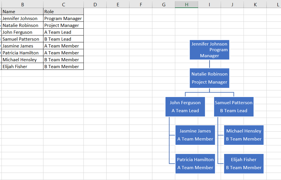
– Repeat Steps 6 & 7 to arrange the rest of the names
– Delete the blank text boxes
Step 9 – Check and format the result
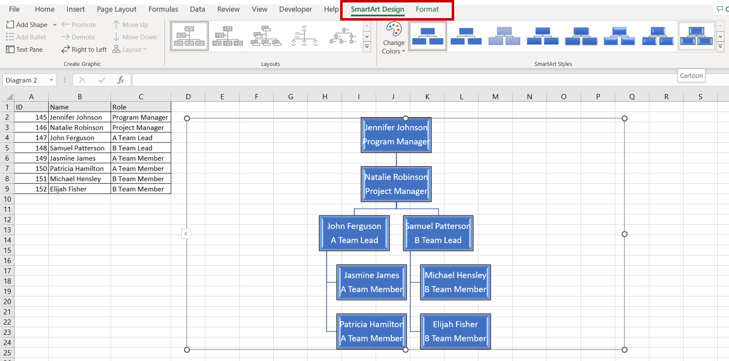
– Format the chart using one of the preset designs under SmartArt Design or customize the chart using the Format options


