
How to create an Array in Microsoft Excel
 By
SpreadCheaters
By
SpreadCheaters
In this tutorial we will learn how to create an Array in Microsoft Excel. Arrays in Microsoft Excel are sets of values organized into columns and rows. They are used to perform calculations and return results for multiple values at once, which can save time and effort compared to performing the same calculation for each value individually.
Microsoft Excel is a popular spreadsheet software application developed by Microsoft Corporation. It is used to organize, analyze, and manipulate data. Excel is widely used for a variety of purposes, including personal finance management, business data analysis, project tracking, and more. Excel provides a powerful set of tools for data analysis, including the ability to create charts, graphs, and pivot tables to visualize your data, and perform complex calculations using formulas and functions. It also supports a wide range of data types, from simple text and numbers to more complex data such as dates, times, and currencies.
Step 1 – Select a Blank Cell
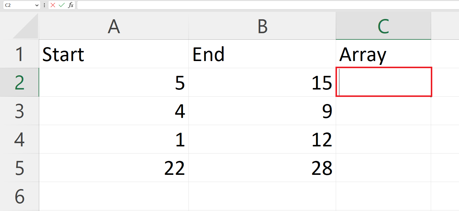
– Select a blank cell where you want to create an array.
Step 2 – Place an Equals Sign
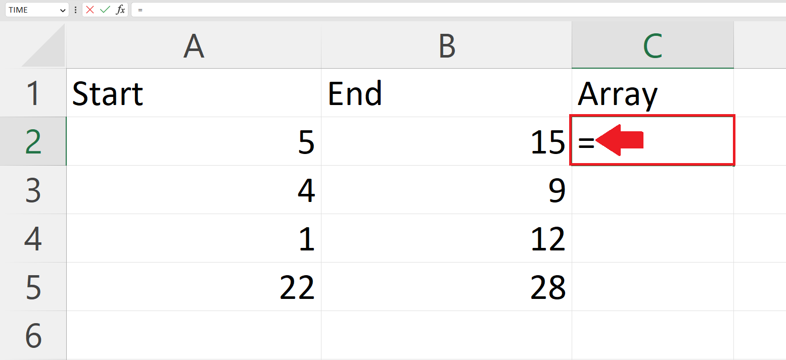
– Place an Equals sign in the targeted blank cell.
Step 3 – Use a combination of ROW and INDIRECT function to Create an Array
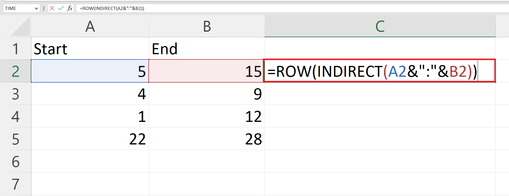
– The formula ROW(INDIRECT(A2&”:”&B2)) is a combination of two Excel functions: ROW and INDIRECT.
– The INDIRECT function takes a string argument and evaluates it as a reference to a cell or a range of cells.
– The ROW function takes a cell reference as an argument and returns the row number of that cell. In this case, ROW(INDIRECT(A2&”:”&B2)) would return the first row number in the range specified by INDIRECT(A2&”:”&B2).
Step 4 – Press Ctrl + Shift + Enter Keys to create the array
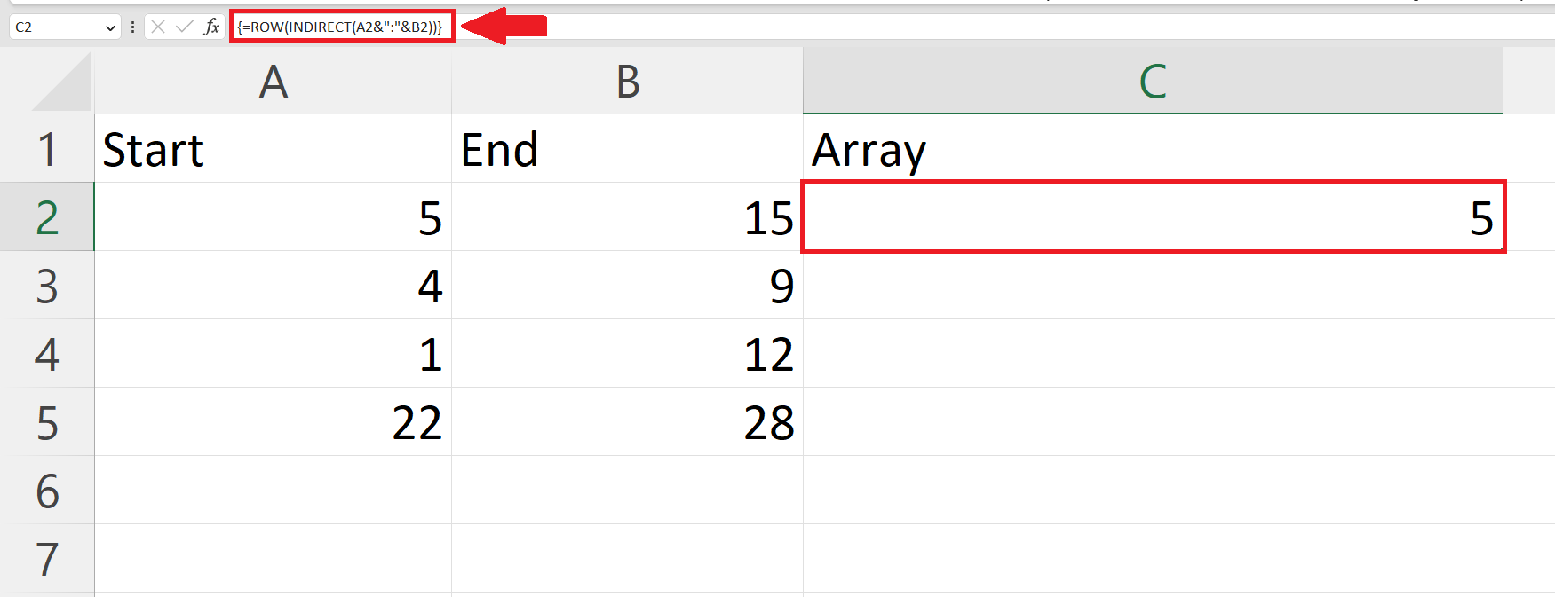
– Press Ctrl + Shift + Enter Keys to create the array.
– Curly brackets will be added in the formula bar when the array will be created.
Step 5 – Viewing the full Array
– Double click on the cell and Press the Enter key to view the full array.
Step 6 – Create an Array for each interval

– Since the functions used above spill the array elements in a single column we can use the TRANSPOSE function before these functions so that Excel spills the array in a single row and other arrays also become visible. So, the formula will become
=TRANSPOSE(ROW(INDIRECT(A2&”:”&B2)))
– Use the “Handle Select” and “Drag and Drop” method to apply the formula to the interval in each row.


