How to create a Vlookup formula in Excel

You can watch a video tutorial here.

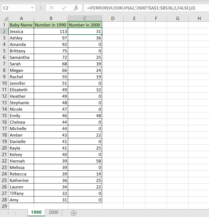
In this example, we have a list of baby names from the year 1990 and the number of children with that name in a particular region. We want to see how many times these names were used in the year 2000. Here the key is the baby name. To do this, we will use the VLOOKUP() function to take each name from the list in the year 1990 and look up the corresponding value from the list in the year 2000.

1. VLOOKUP() function: this searches for a value in the leftmost column of a range, and returns the value in the column specified from the row of the match in the range.
   • Syntax: VLOOKUP(lookup_value, table_array, col_index_num, range_lookup)
   • lookup_value: the cell reference of the first value in the key column from Table 1 (Name)
   • table_array: the range of Table 2 which is made constant with the addition of dollar signs ($)
   • col_index_num: the number of the column in Table 2 that has to be retrieved (1 i.e. the Name)
   • range_lookup: TRUE will return an approximate match, FALSE will return an exact match
2. A few things to keep in mind when using Vlookup:
   1. The key must always be in the left-most column of the table being referenced
   2. The table that is being referred to must always be sorted on the key, in ascending order
   3. It is better that the being referred to has unique values or else this function may not return the desired result

Vlookup is one of the most useful functions in Excel when it comes to comparing data from multiple tables or ranges. As long as the tables share a common field or ‘key’, data from both tables can be easily compared.

Step 1 – Start typing the formula

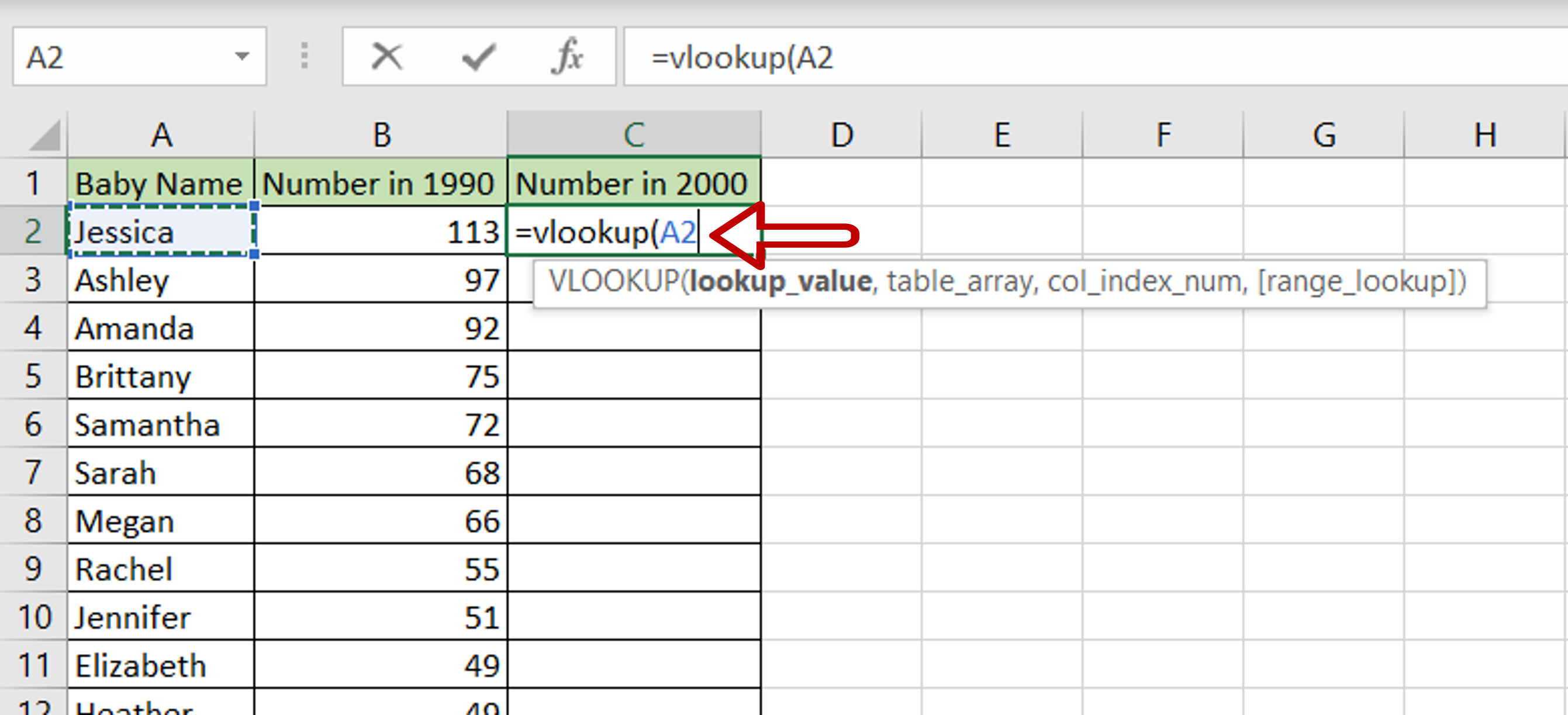
– Select the cell where the result is to appear
– Start typing the formula using cell references:
=VLOOKUP(Baby Name,

Step 2 – Reference the second table

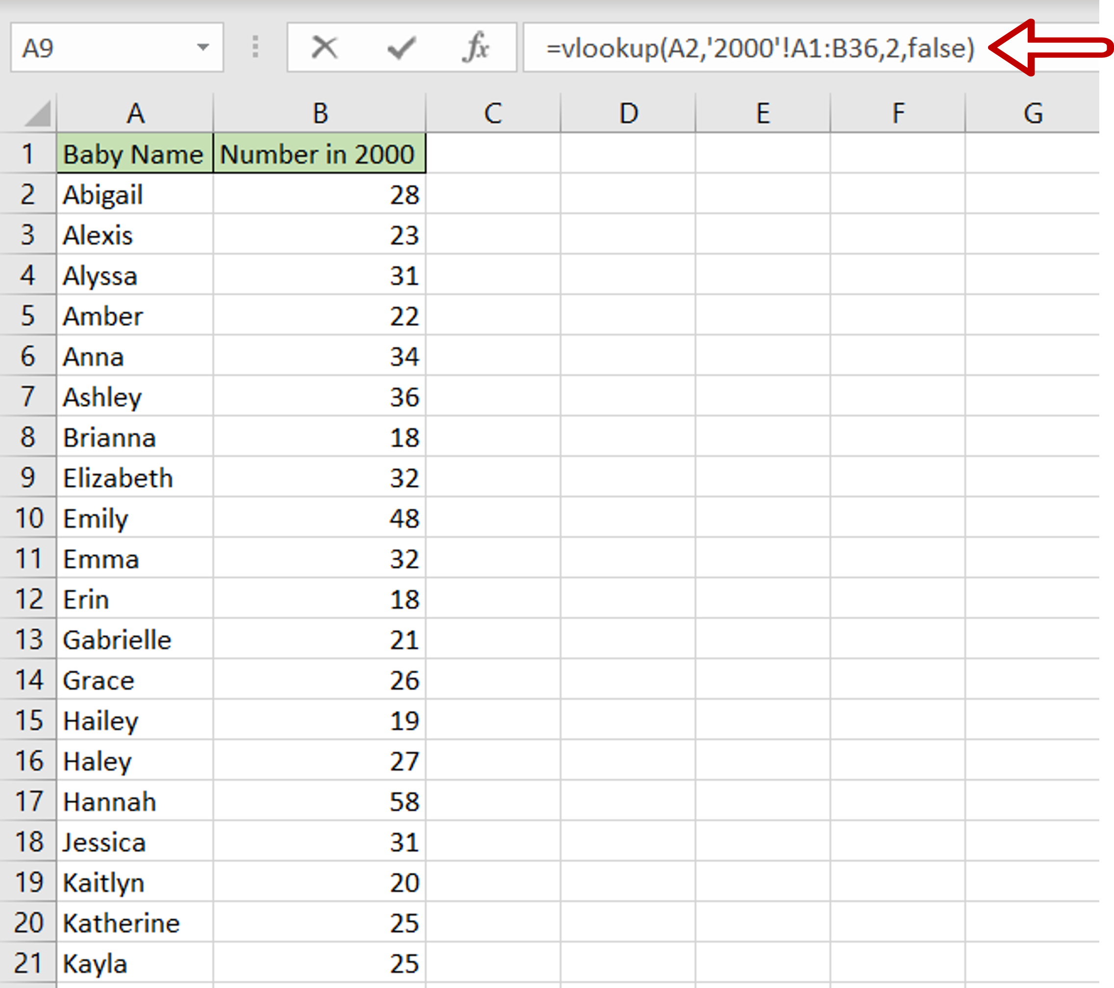
– Go to the second table and select the range of the data that is being compared
– The range will be added to the formula with the file and sheet name
– Complete the formula:
= VLOOKUP(Names, range in the second table, 2, FALSE)
– The col_index_num is set to 2 because we want the value in the second column
– Press Enter

Step 3 – Make the range constant

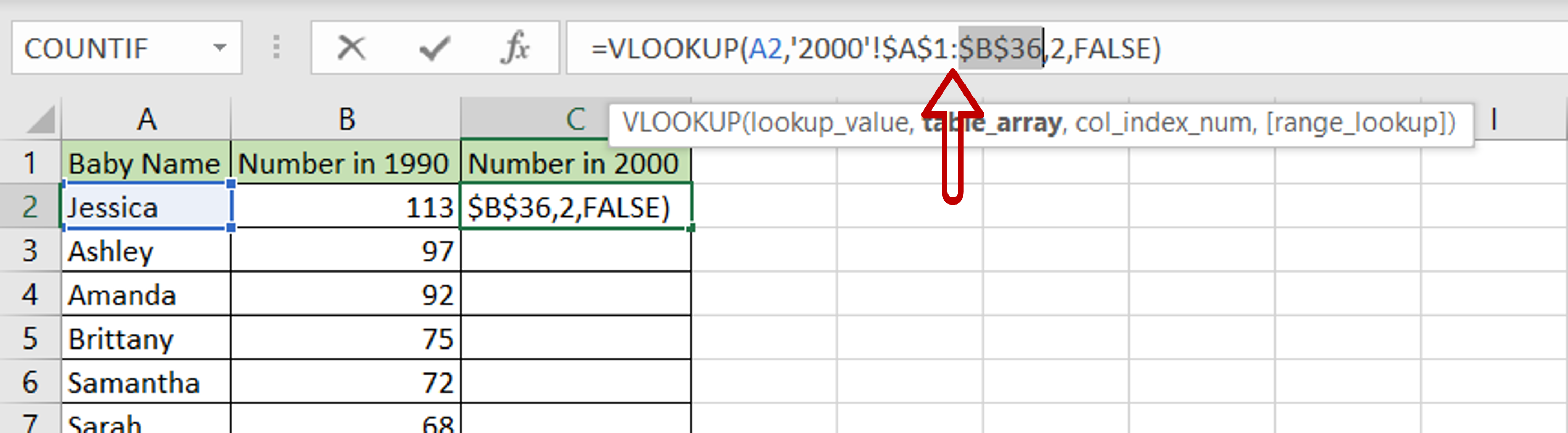
– Select the cell that has the formula
– Press F2 to enable the cell for editing
– Select the cell references of the range being referred to and press F4
– This inserts dollar signs ($) that make the range constant

Step 4 – Enhance the formula to handle errors

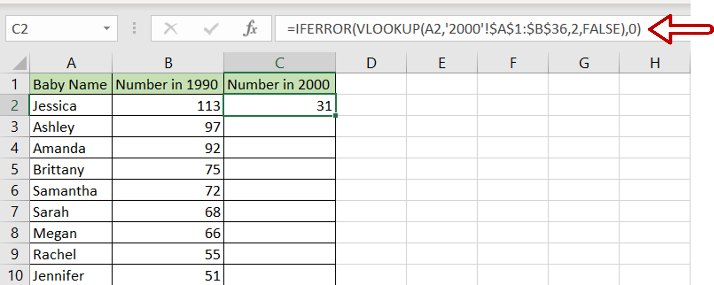
– If the lookup function cannot find a match in the range being referred, an error message will be returned i.e. #N/A
– Change the formula to display a zero if a match cannot be found:
= IFERROR(<vlookup formula>,0)

Step 5 – Copy the formula

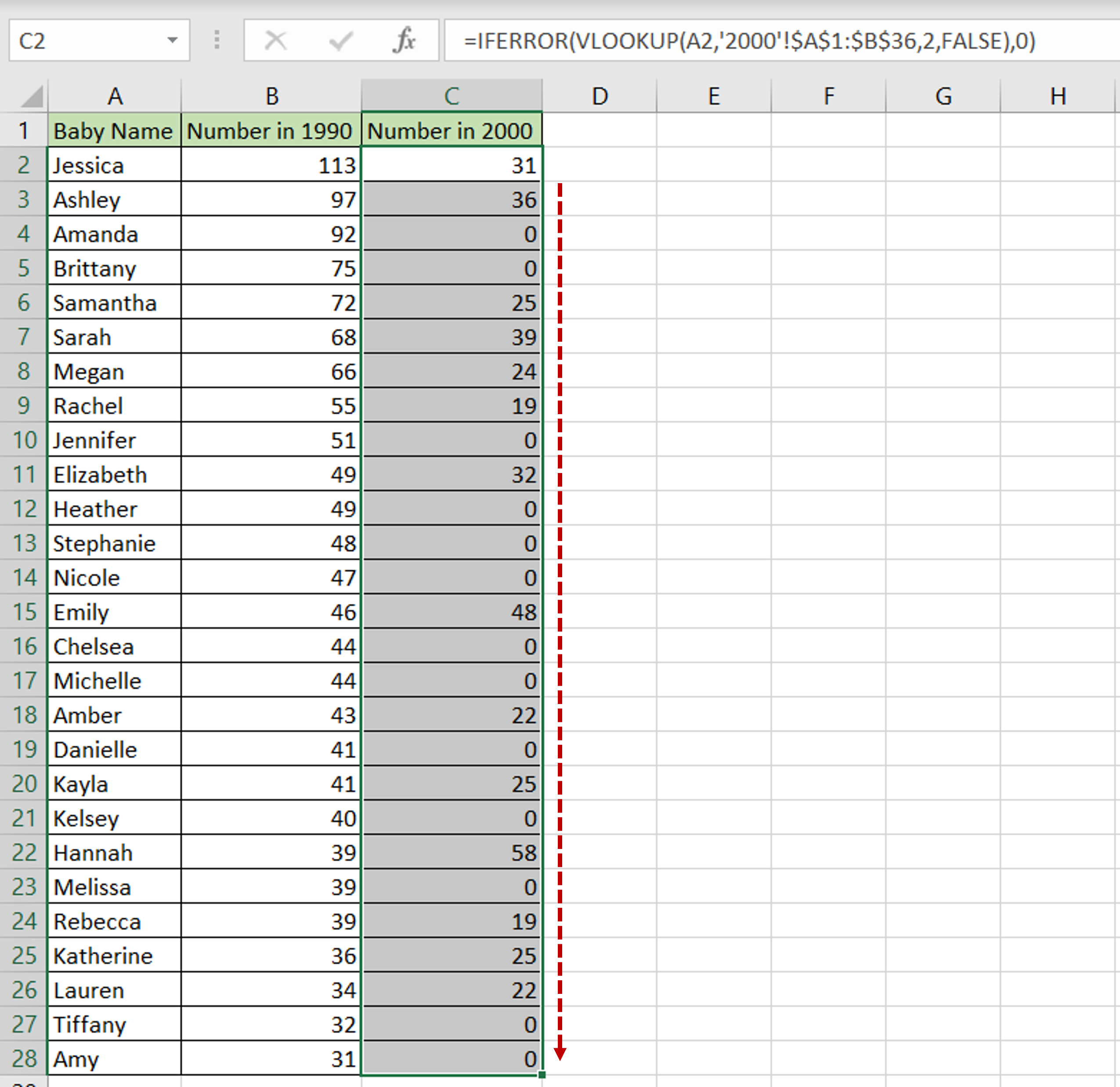
– Using the fill handle from the first cell, drag the formula to the remaining cells
OR
a) Select the cell with the formula and press Ctrl+C or choose Copy from the context menu (right-click)
b) Select the rest of the cells in the column and press Ctrl+V or choose Paste from the context menu (right-click)

Step 6 – Check the result

– The number of times that the name was used in 2000 appears in the column
– A zero is displayed for the names that were not found in the list for the year 2000