
How to create a blank pivot table in Excel
 By
SpreadCheaters
By
SpreadCheaters
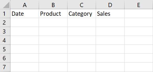
Our data comprises a report from a store that includes information such as the date, the names of products sold, their respective categories, and the number of sales for each product on a given day. To create a blank pivot table for this data, we will choose the relevant table headers and use the pivot table option to generate a summary table. This will enable us to explore and analyze our sales data from various perspectives, providing valuable insights into our business performance.

A blank pivot table in Excel is a table that has no data or fields yet but is structured in a way that allows you to summarize and analyze large amounts of data quickly and easily. The importance of a blank pivot table in Excel lies in its ability to help you quickly make sense of large and complex data sets. By summarizing and analyzing data in different ways, you can identify trends and patterns that might not be immediately apparent from the raw data.
Step 1 – Select the range of cells

– Select the blank range of the cell including the headers of the pivot table
Step 2 – Click on the Pivot Table option
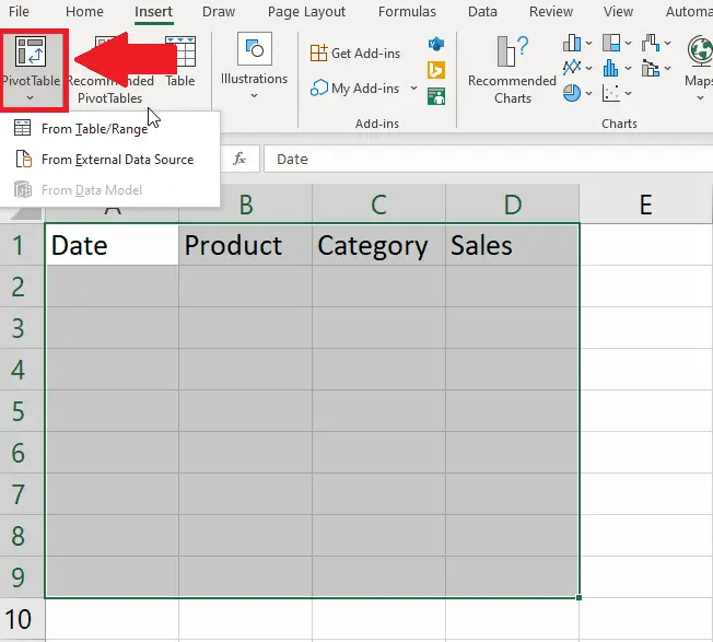
– After selecting the range of cells, click on the Pivot table option in the Tables group of the Insert tab and a drop-down menu will appear
Step 3 – Click the From table range option
– From the drop-down menu, click on the From Table range option and a dialog box will appear
Step 4 – Click on the New Sheet option
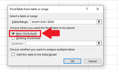
– In the dialog box, click on the check box behind the New sheet option
– If you want to form the pivot table on the same sheet, click on the Existing Sheet option and type the range of the table in the box next to the location option
Step 5 – Click on OK

– After selecting the location of the pivot table, click on OK at the end of the dialog box to get the required result


