
How to count highlighted cells in Excel
 By
SpreadCheaters
By
SpreadCheaters
You can watch a video tutorial here.

When formatting cells in Excel, you may highlight certain cells based on the value of the cell. You may then need to count the number of cells according to their color. In this example, you would like to count the days on which the sales amount is less than the average and these have been highlighted.
Step 1 – Turn on the in-column filters
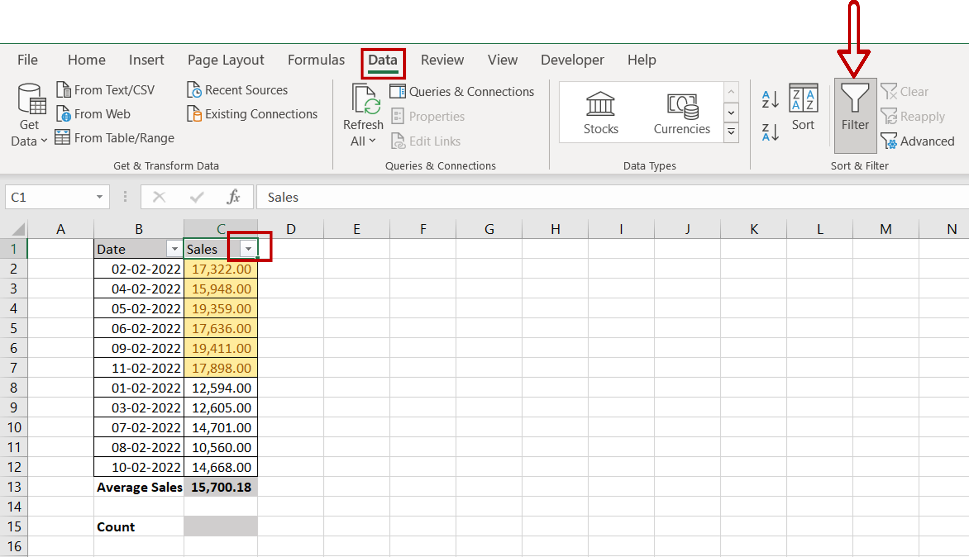
– Go to Data > Sort & Filter
– Click the Filter button
Step 2 – Choose the filter
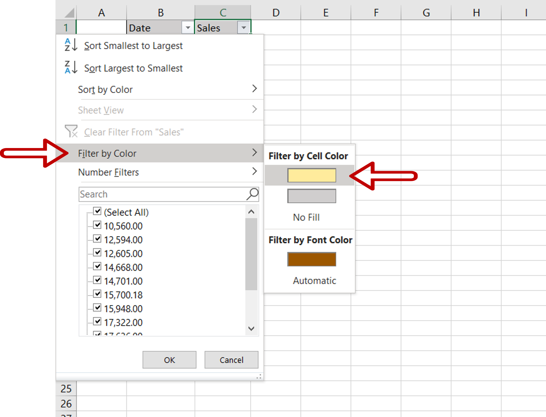
– On the filter drop-down menu, choose Filter by Cell Color
– Choose the color of the highlighted cells
Step 3 – Count the filtered cells
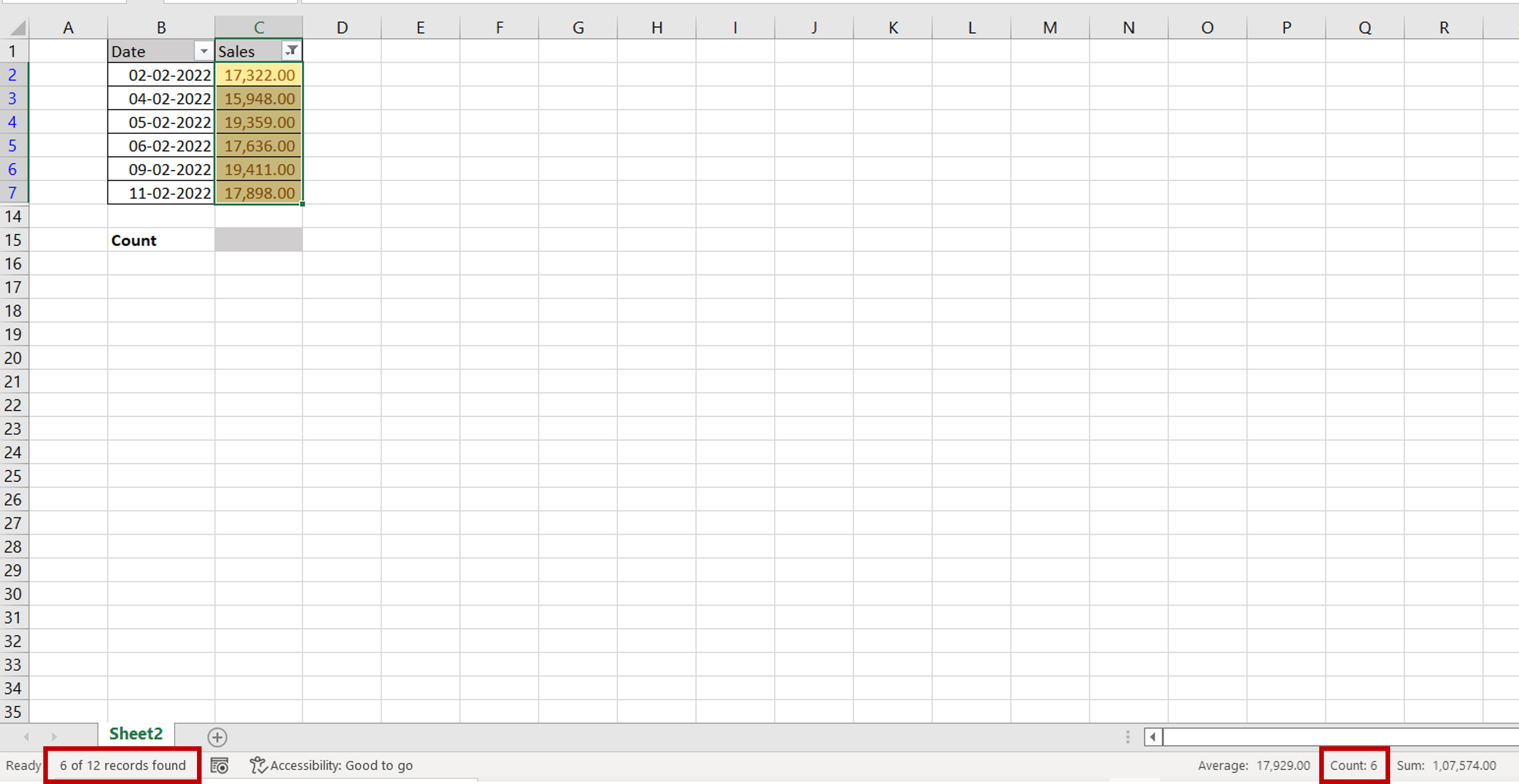
– On the bottom left of the sheet, the number of filtered cells will be displayed
– Select the filtered cells and check the bottom left of the sheet where the count of the cells will be displayed
Step 4 – Create the Subtotal() function
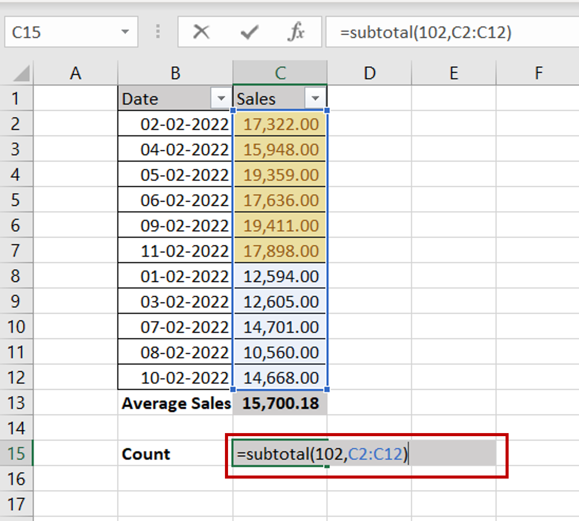
– From the filter menu, select Clear Filter from “Sales” to remove the filter
– In a cell below the table enter the formula:
=subtotal(102, <range of the ‘Sales’ column>)
Note: 102 represents the COUNT function. For a full list of numbers that can be used with Subtotal(), refer https://support.microsoft.com/en-us/office/subtotal-function-7b027003-f060-4ade-9040-e478765b9939
Step 5 – Filter the data
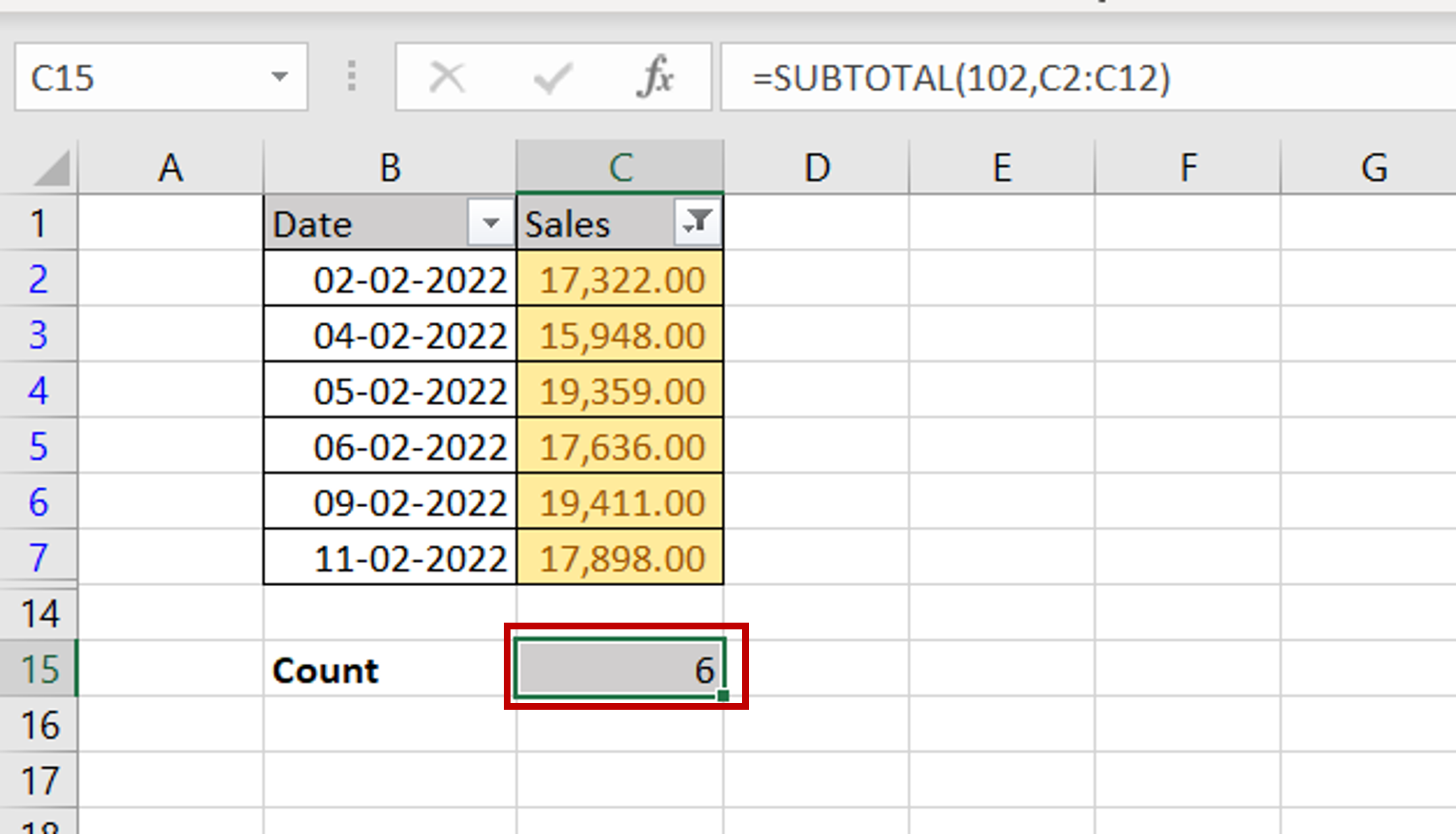
– Apply the color filter again
– The count of the highlighted cells will be displayed


