How to count colored cells in Excel

Some data analysts like to present their data in a very aesthetic way and therefore they use colorful themes to differentiate one type of data from others. In such cases often there is a requirement to count the cells that have similar colors. 

Microsoft Excel doesn’t provide us with a straightforward method to achieve this goal. However, we can get it done by using the following methods;

• Filter and SUBTOTAL
• Use the FIND tool

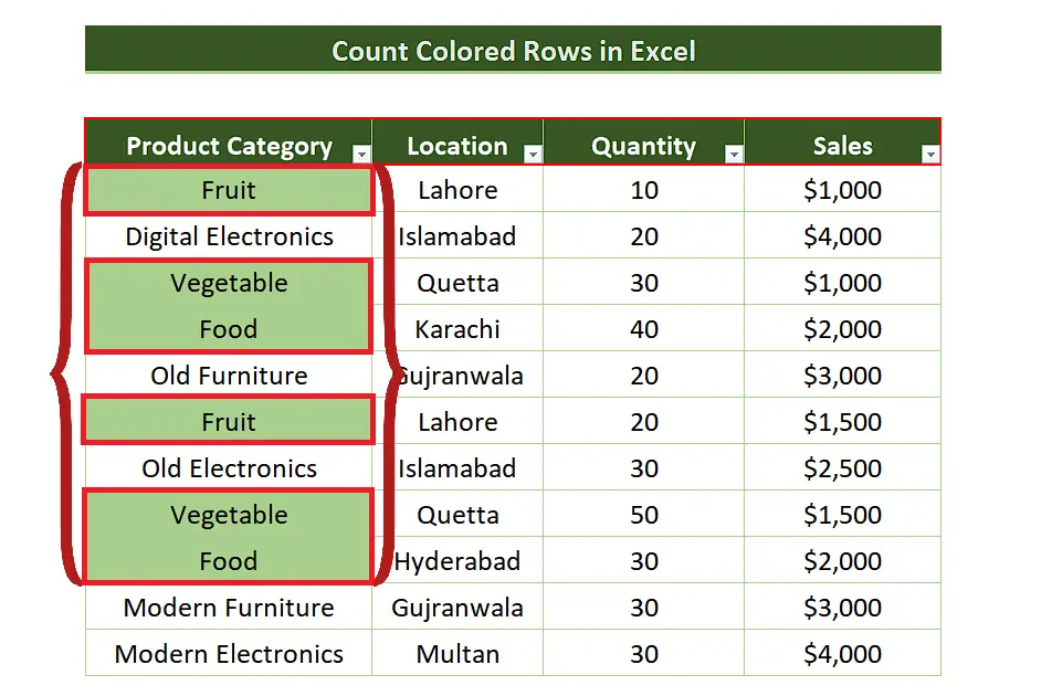
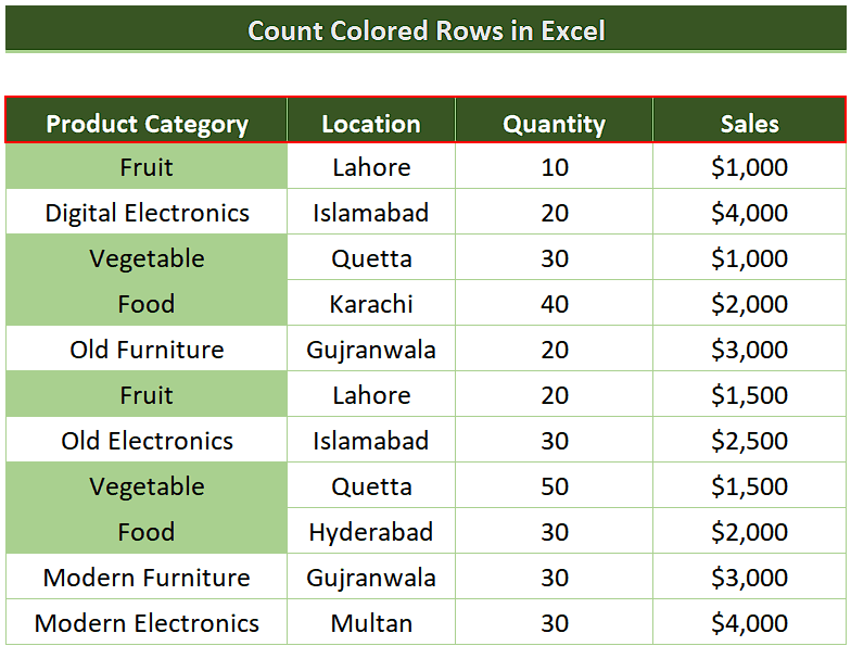
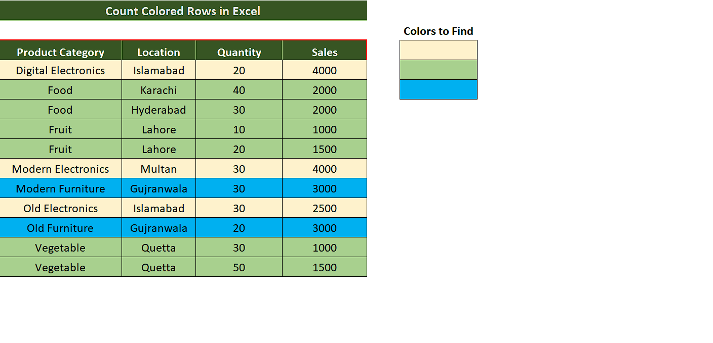
We are going to learn how to Count Colored Rows by all above mentioned methods in Excel. Let’s take a look at the following sales dataset.

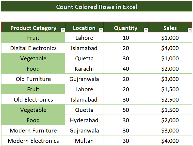
Step 1 – Apply the filter using shortcut key CTRL+SHIFT+L

• Select a cell inside your dataset.
• Use the shortcut key to apply a filter to the dataset by pressing CTRL+SHIFT+L.
• This will apply the filter to all columns in the data range automatically.

• The same thing can also be done by going to the Sort & Filter option in the Editing group on the Home tab from the list of main tabs in Excel.

Now that we have applied the filter to our data, we can use it as per our requirements to see only the data that we are interested in. Let’s assume that we wish to see the sales data of eatables which are colored green in the dataset such as Fruit, Vegetable and Food items only from the Product Category column. So, let’s use the filter options to get it done.

Step 2 – Use Filter by Color to filter rows in Excel

• We’ll go to the column header of interest, which in our case is the Product Category and click on the dropdown arrow.
• This will open up new options and we’ll click the Filter by Color option this will give us the option to choose between all the cell colors available in our data range. Since we have only one color i.e. (green) therefore, we’ll see this color and No fill option. 
• We’ll choose the   (green)  option and all our data will be filtered and we’ll see only the green colored cells.

Step 3 – Use SUBTOTAL function to count the filtered cells

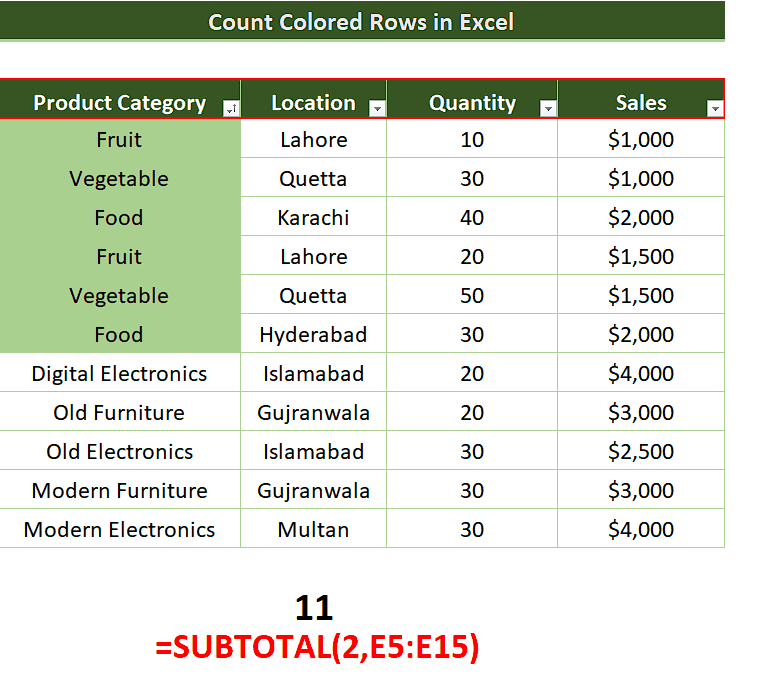
• Now we’ll use the subtotal function to count the number of rows as a result of application of the color filter. We’ll use the following simple formula;

=SUBTOTAL(2,E5:E15)

• In the above formula, we are counting the colored cells indirectly by counting the sub rows that contain numeric data. This will give us the count of the rows only which are colored.

This is how we can count the colored rows in Excel by using Filter and SUBTOTAL together.

Method 2 – Use the FIND tool to count colored rows

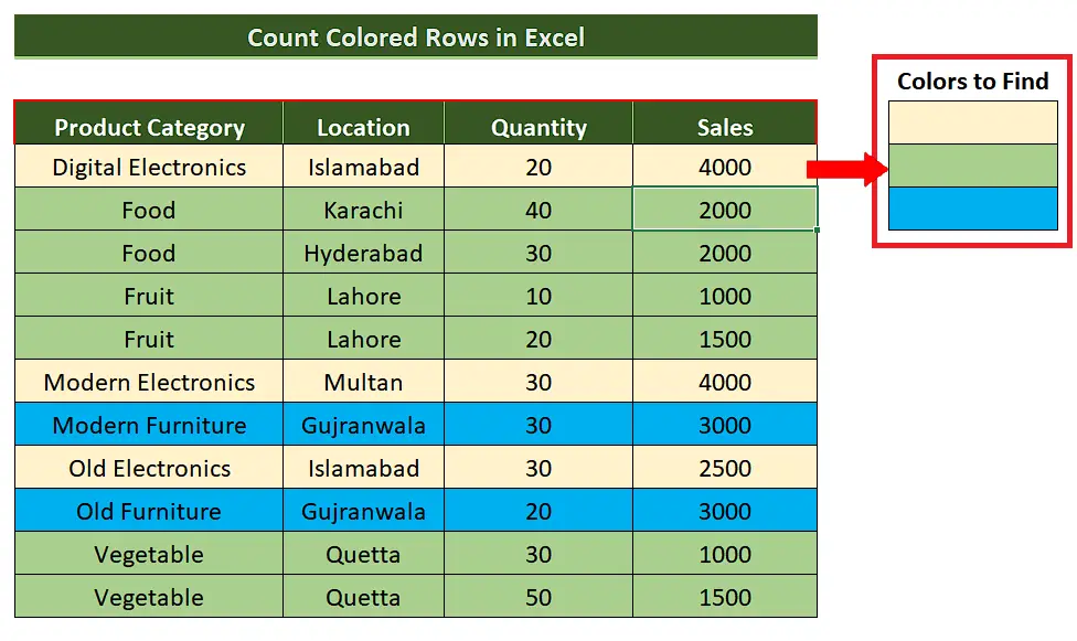
We can achieve the goal of counting the number of colored rows in Excel by using the FIND tool as well. For this we should have a color map in cells. This will help us in choosing the type of colored rows to find and count. Let’s see the dataset shown above.

Let’s see how it can be done by following the steps mentioned below;

Step 1 – Press CTRL+F to open Find dialog box and set color format

• To use the find tool, press the CTRL+F shortcut key to open the options dialog box.
• Now click on Format dropdown to open up the options.
• Click on Choose Format From Cell and now click on the cell which should be filled with the color your data rows have.
• Now select the data column from which you wish to count rows with a specific color.
• Press Find All option and you will see the number of cells with your selected color at the bottom left corner of the dialog box.
• You can also see the cell addresses which have the same color as your search format.