How to count cells with value Greater than Zero in Excel

In this tutorial we will learn how we can use Excel’s built-in “COUNTIF” function to calculate the number of cells greater than Zero. A better way to understand how countif works in such situations, is to first understand the structure of the function and the parameters it requires.

Structure of COUNTIF

The standard syntax of countif function in excel is shown below;

=COUNTIF(range, criteria)

• range (where to look in for something)

A range can be a single column with multiple rows or it could consist of multiple columns and multiple rows. For example “A1:A14”. This will tell the formula to search through column A till the 14th row.

• criteria (what to look for)

Criteria will always be a special logical condition depending upon the situation and the nature of values that we are looking for. In the example at hand we will be looking for all those cells which have values greater than ZERO.  We will use a special logical condition in the formula for Excel to count those cells which have values greater than ZERO.

Implementing the Formula on an Actual Data Set

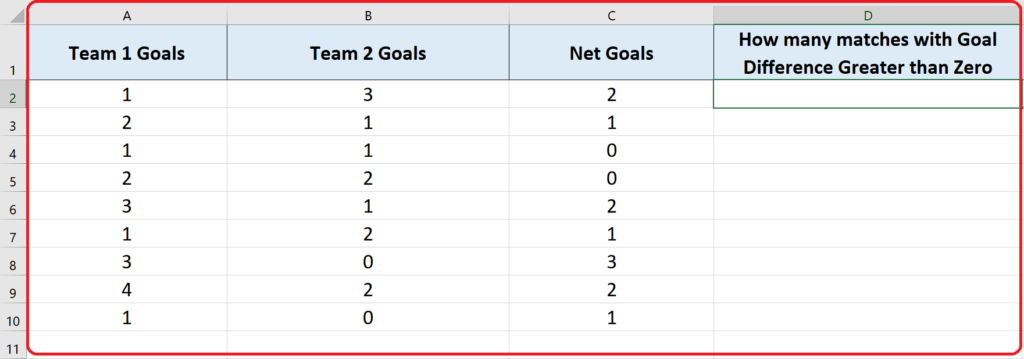
Let’s take an example data set and find out the number of cells having values greater than ZERO in it. So let’s consider the data set shown above.

Our data set contains the results of some soccer matches. It has the number of goals scored by each team during a single match and it calculates the net number of goals scored in each match as well. Suppose we want to know the number of matches which were not drawn.

To achieve this we will count the number of matches in which the net goals were more than ZERO. This will give us the desired result. In this case we can use the countif formula to find a solution to our problem. Let’s do this by following these step;

When we work with practical data sets using Excel, every now and then we have to count those cells which have values greater than Zero. Excel has a very easy way to find out the number of cells greater than Zero within a specific range.

Step 1 – Implement the formula in a suitable cell

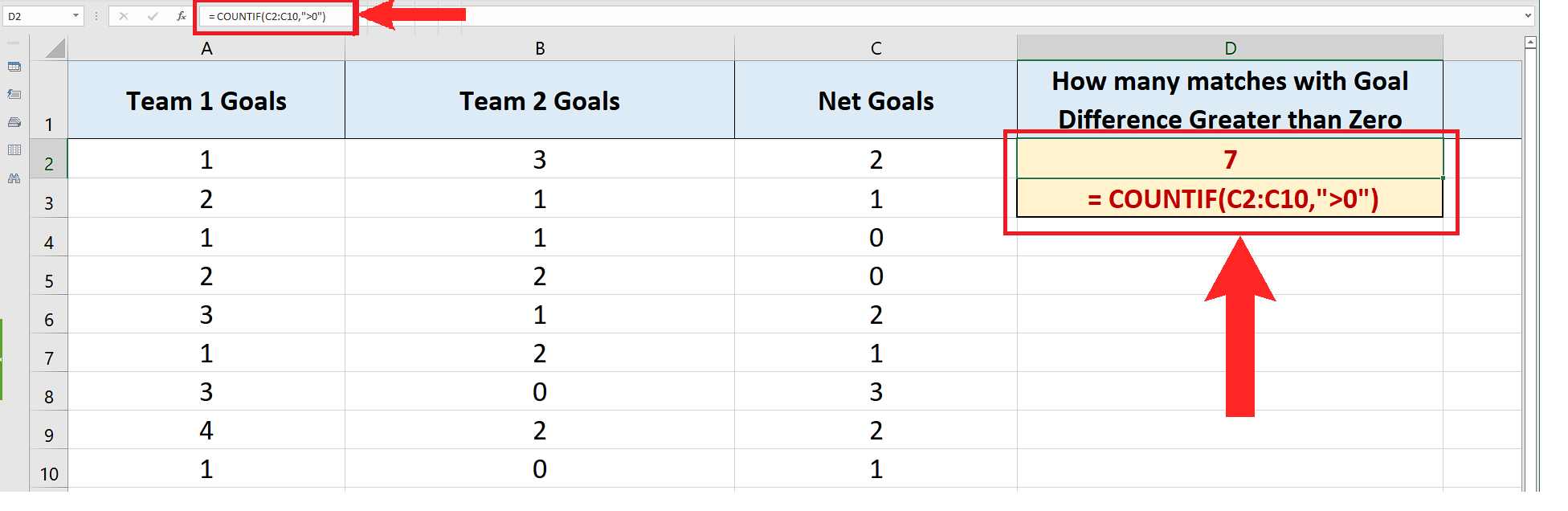
– Choose a suitable cell where you wish to implement the formula. In this case we have chosen D2 to implement this formula.

– Use the following formula in that cell and press enter key.

= COUNTIF(C2:C10,”>0″)

– The desired result will be displayed in this cell as soon as you will press the enter key as shown in the picture above.

Simple, wasn’t it. We used COUNTIF with a special condition to count all rows in column C which had a value greater than ZERO and successfully found out that there were 7 matches in which we got a result and the match was not drawn.

Breakdown of the Logical Condition used inside the formula

We used the formula COUNTIF(C2:C10,”>0″). Let’s see how we told Excel where to look and what to look for. 

• The first parameter C2:C10 tells Excel that the data range in which we are going to look for something is in column C and from row 2 to row 10 only.

• The second parameter was “>0”. This condition tells Excel to look for all those cells that have values greater than ZERO. When Excel finds a cell meeting this condition it increases the value of the counter. Our data set had seven cells which had values greater than ZERO in that range so the result was 7 as we desired.