
How to copy paste formulas in Excel
 By
SpreadCheaters
By
SpreadCheaters
Copy and paste is a very basic function of Excel used to duplicate content or move content from one location to another. This can be useful for a variety of reasons, such as copying a formula to multiple cells to perform the same calculation in each cell, or copying a set of data from another source and pasting it into an Excel spreadsheet.
In this tutorial, we will learn how to copy and paste formulas in Excel. We can do this by the following methods.
- Copy and paste the formula down the column with changing references
- Copy and paste the formula down the column without changing references
- Copy and paste the formula to non-adjacent cells
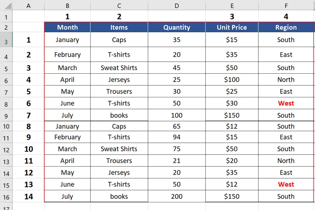
Let’s see how to implement these methods in the steps below. Let’s look at the dataset at hand. It consists of sales data from various regions.
Method 1: Copy and paste formula to whole column with changing references
Let’s calculate the total cost of each item by copying the formula from the first cell. In this method we’ll use the changing references because we need to use the unit cost of each item individually.
Step 1 – Calculate the total cost of first item
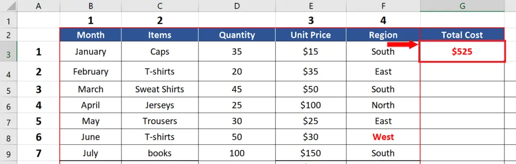
- Choose a suitable cell for this purpose and implement the formula =D3*E3, because the number of items is in D3 and unit cost is in E3.
- Press Enter to implement the formula and get the first result.
Step 2 – Copy the formula down the whole column
- Now move the mouse to the bottom right corner of the cell where you implemented the formula.
- Wait till the mouse turns into a black plus sign. This is when you need to double click and the formula will be automatically copied down the whole column.
- Alternatively, you can select the first cell where you implemented the formula and press CTRL+C. Then select the whole data range manually and press CTRL+V. In case you have a very big dataset then using these shortcuts is not a recommended solution. Use double clicking the fill handle in this case.
Method 2: Copy and paste the formula down the column without changing references
In this method we’ll convert the total sales of each item from Dollars to Euros and therefore, we’ll need to implement the same conversion rate for each value. We’ll use a fixed cell reference which will have the conversion rate in it and then simply multiply all values with it one by one. The conversion rate will be written in the cell H1 for our example case. We’ll fix this cell’s reference by using the F4 command. Let’s do this by following the steps below.
Step 1 – Write the conversion rate in suitable cell
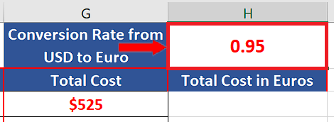
- Choose a suitable cell, for our example, we’ll use H1.
- Enter conversion rate for USD to Euro i.e., 0.95.
Step 2 – Write the formula in the first cell and fix reference for H1
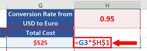
- Now write the formula =G3*H1 in the cell H3.
- Keep the mouse cursor over H1 and press F4 key. This will change the formula to =G3*$H$1. It means that the reference for H1 has been fixed now and it will not change when we copy and paste the formula down the whole column.
Step 3 – Copy the formula down the whole column
- Now move the mouse to the bottom right corner of the cell where you implemented the formula.
- Wait till the mouse turns into a black plus sign. This is when you need to double click and the formula will be automatically copied down the whole column. However, this time the cell value of H1 will not change while copying down the formula.
Method 3: Copy and paste formula to non-adjacent cells
This time around, let’s calculate the total cost of T-shirts only by copying the formula from the first cell to only those cells where required. Let’s do it by following the steps below.
Step 1 – Calculate the total cost of first occurrence of T-shirt item
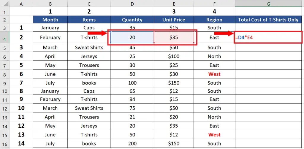
- Write the formula =D4*E4 in G4, because the first occurrence of a T-shirt is in row 4.
- Press the Enter key to calculate the total cost of the first instance.
Step 2 – Copy the formula to the selected cells
- Select the cell where you implemented the formula and press the shortcut key CTRL+C to copy the formula.
- Hold the CTRL key and keep selecting the cells where you wish to paste the formula. In our case these cells will be G8, G11 and G15.
- Now press CTRL+V and the formula will be pasted in only those selected cells.
- To check the authenticity of the formulas, we can go to each cell and press F2 to see which cells are being used in the formula as shown below.


