How to copy every other row in Excel

Copying every other row in Excel means selecting every other row in a range or table and copying its contents to another location. This is often done when you want to extract a subset of data from a larger dataset. The importance of copying every other row in Excel depends on your specific use case. It can be a useful technique when you want to analyze a subset of data, but it may not be necessary in every situation. 

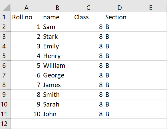
Our dataset includes information about students, including their names, class, section, and roll number. We want to divide the students into two groups based on their roll number. Specifically, we want to create a group of students with odd-numbered roll numbers and copy their data to a new sheet. This will give us a separate sheet containing data only for Group 1. To achieve this, we need to select alternate rows and copy them to the new sheet.

Method 1: Copy Every Other row using the CTRL key 

Step 1 – Select the first row

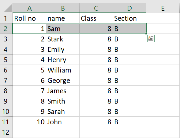
• Select the first row that you want to copy

Step 2 – Select the Other rows

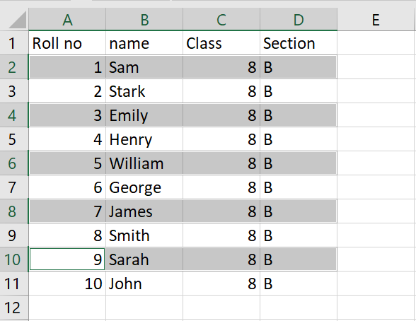
• After selecting the first row, press the CTRL key
• While pressing the CTRL key, select the other rows that you want to copy

Step 3 – Copy the rows

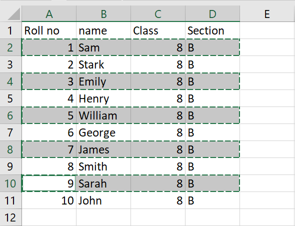
• After selecting the rows you want to copy, press the CTRL+C keys to copy the selected rows

Step 4 – Select the cell

• Click on the cell where you want to paste the copied row
• Here we have selected a cell of the new sheet, you may select any other location we want

Step 5 – Paste the Selected rows

• After selecting the location where you want to paste the copied rows, press the CTRL+V keys to paste the rows

Method 2: Copy Ever Other rows using the Find and Select option

Step 1 – Type an Alphabet in a new column

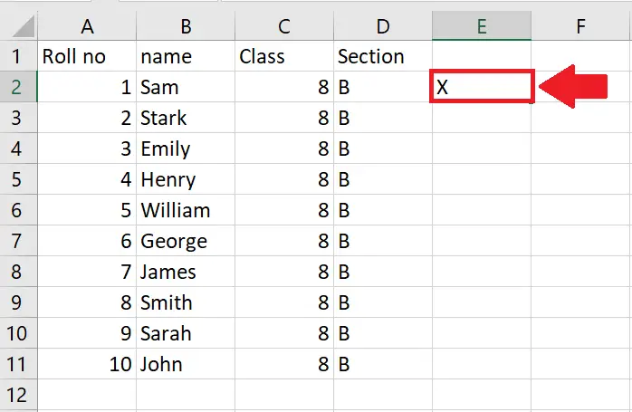
• Type any alphabet in the column next to your dataset 
• Here we typed “X” as the alphabet 

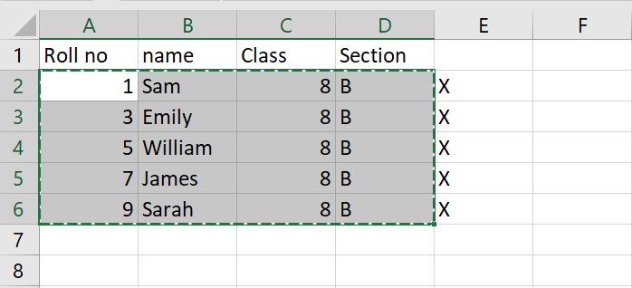
Step 2 – Drag the Written alphabet

• Select the cell containing the alphabet and the cell next to it(blank cell)
• After selecting these 2 cells, drag them till it is required
• And the pattern will appear in the column

Step 3 – Click on the Find and Select option

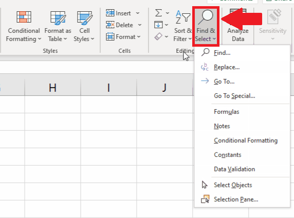
• Select the range of cells
• And click on the Find and Select option and a dropdown menu will appear

Step 4 – Click on the Go To Special option

• From the drop-down menu, click on the Go To Special option and a dialog box will appear

Step 5 – Click on the Blanks option

• In the dialog box, click on the checkbox behind the blanks option

Step 6 – Click on Ok

• After clicking on the blanks option, click on OK at the end of the dialog box 
• And the blank cells of the columns will be selected

Step 7 – Open the context menu

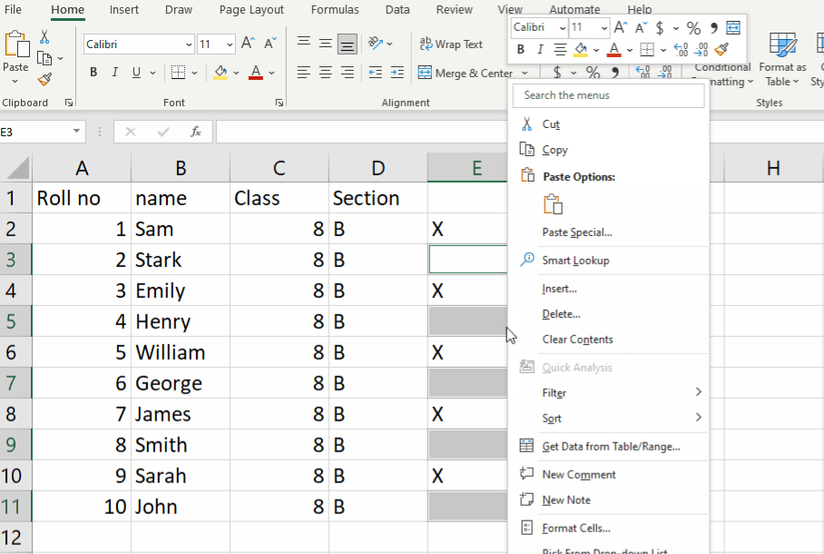
• After selecting the blank cells, right-click on any selected cell, and a context menu will appear

Step 8 – Click on the Delete option

• In the context menu, click on the delete option and a dialog box will appear

Step 9 – Click on the Entire row option

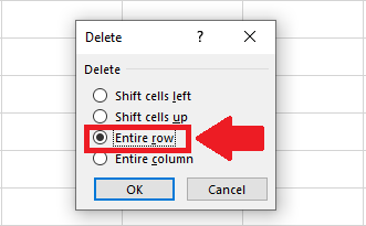
• From the dialog box, click on the Entire row option

Step 10 – Click on Ok

• After selecting the Entire row option, click on OK 
• And the row containing the blank cells of the selected column will disappear

Step 11- Copy the range of cells

• Select the range of cells that will appear after deleting the rows, except the column of containing the alphabet(X)
• Press the CTRL+C keys to copy the range

Step 12 – Select the Cell

• After copying the range, click on the cell where you want to paste the copied range

Step 13 – Paste the copied range

• After selecting the cell where you want to paste the range, press the CTRL+V key to get the required range 

Method 3: Copy Ever Other row using the Filter option

Step 1 – Type the Combination of functions

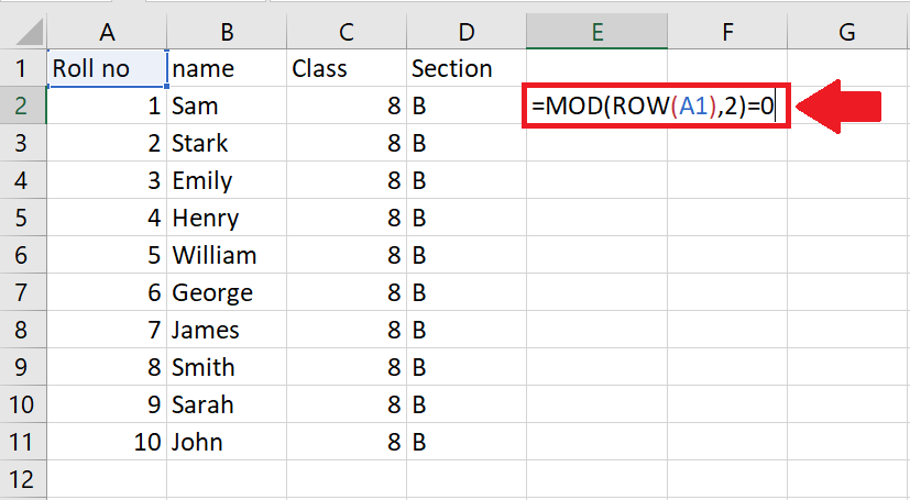
• Click on the cell next to your dataset and type the combination of formulas:
• =MOD(ROW(A1),2)=0

Step 2 – Press the Enter key

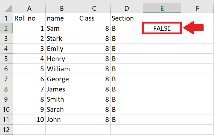
• After typing the functions, press the Enter key and a False will appear

Step 3 – Drag the Cell

• After getting the result of the function, drag the cell the required cell of the column to apply the functions on the complete column
• And a pattern of FALSE and TRUE will appear in the column

Step 4 – Click on the Sort and Filter option

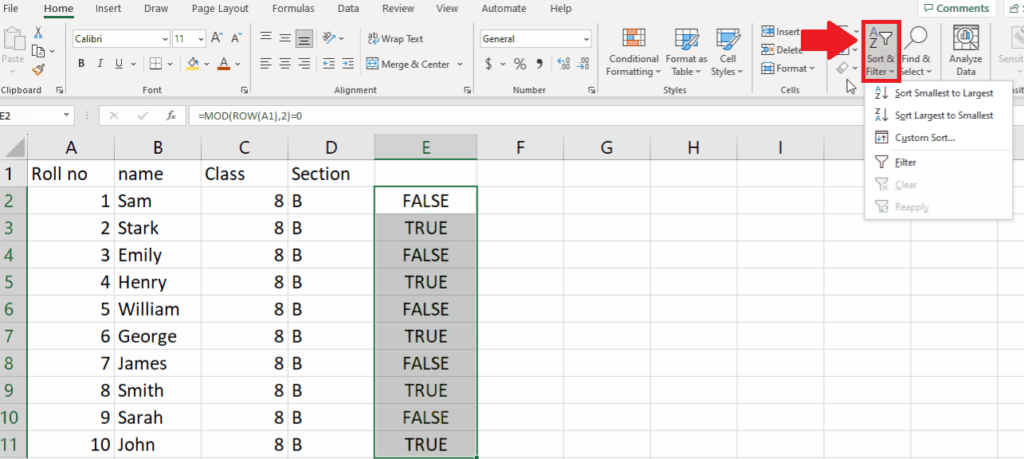
• After applying the function on the complete column, select the column
• And click on the Soert and Filter option, and a drop-down menu will appear

Step 5 – Click on the Filter option

• In the drop-down menu, click on the Filter option and a filter symbol will appear on the first cell of the selected column

Step 6 – Click on the filter Symbol

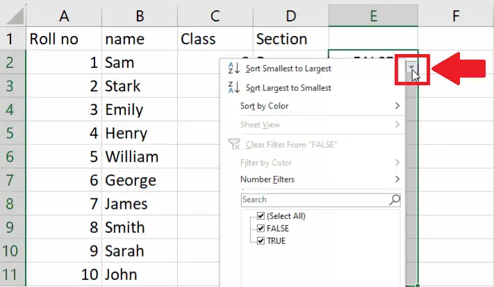
• Click on the filter symbol of Filter at the first cell of the column and a dropdown menu will appear

Step 7 – Click on the checkbox

• From the dropdown menu, click on the FALSE and the rows having the FALSE in their cells will appear while the other rows will disappear

Step 8 – Select the range of cells

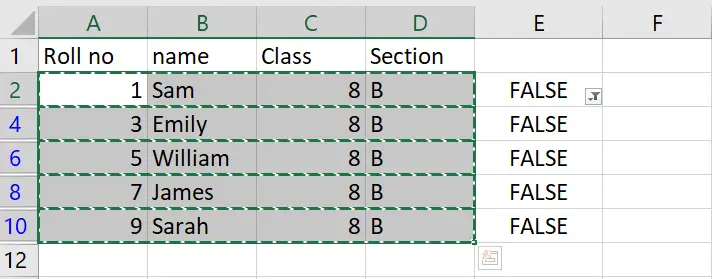
• When the range of cells will appear after applying a filter, copy the range
• To copy it, press the CTRL+C keys

Step 9 – Select the cell

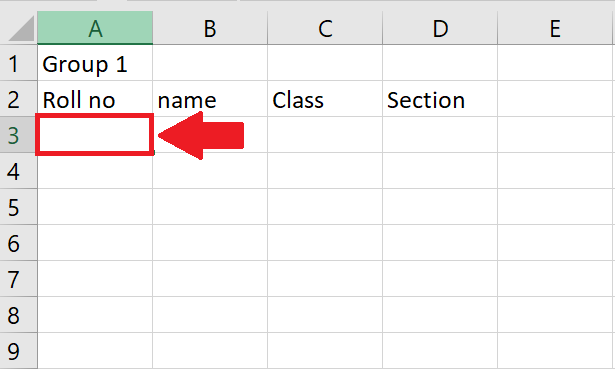
• Click on the cell where you want to paste the copied row
• Here we have selected a cell of the new sheet, you may select any other location 

Step 10 – Paste the Selected rows

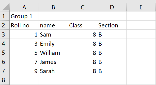
• After selecting the location where you want to paste the copied rows, press the CTRL+V keys to paste the rows