How to convert the formula to text in Excel
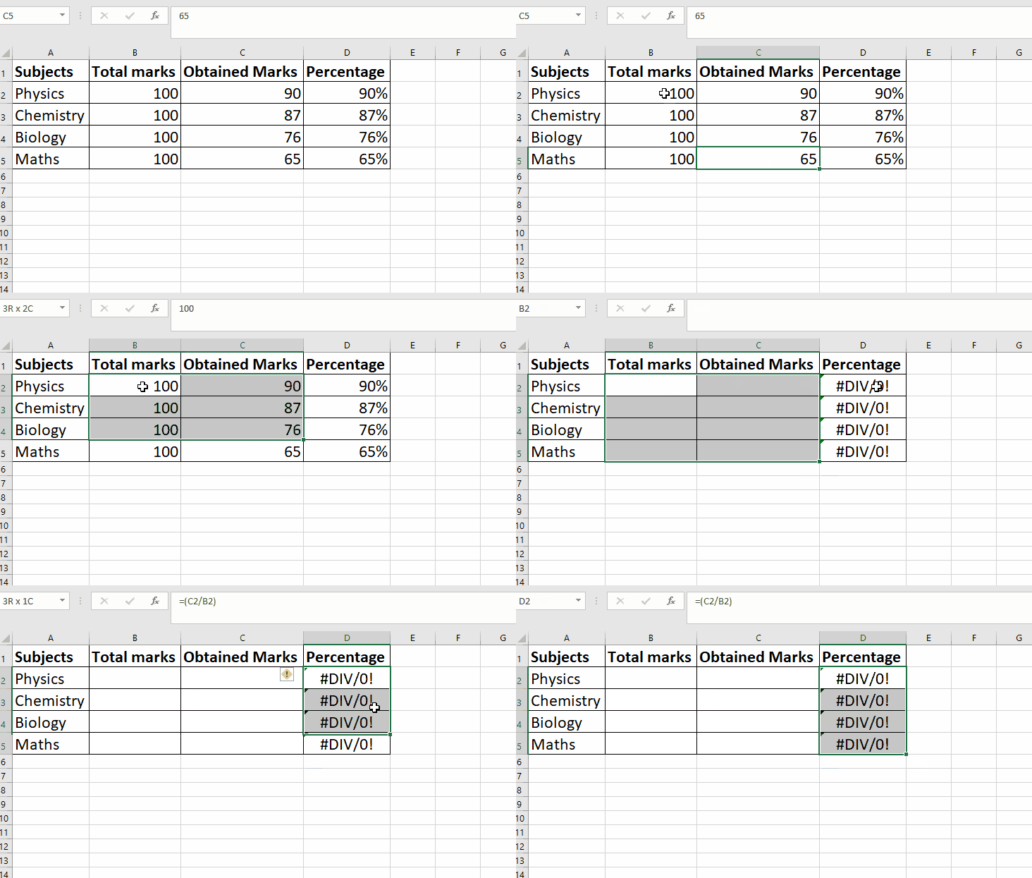
Excel provides powerful tools and features for data manipulation, data visualization, data computation, etc. For this purpose, we use many different types of formulae. In our daily use of excel, we face a problem, when a formula is applied between two columns. We can not delete / hide that particular column even if it isn’t necessary. Therefore, it impacts the overall presentation of the sheet and the results as well. Most of the time it gives #REF or #DIV/0! errors. if we delete the column which is used inside the formula.

The above-mentioned problem can be resolved by converting the formulae to text and this tutorial will guide you on how to convert the formula to text in Excel.
Excel allows us to convert the applied formula and the result values into text. For instance, we have a data set of mark sheets with a percentage column. We only need the percentage column in our further queries and we want to hide or delete the total marks and obtained marks column. We will use a Paste special option for it. Using this option we can paste the value and convert the formulae into text. Below are the two methods by which we can use the paste special tool.
Method 1 – Use the paste option
In this method, we will use the paste special button to convert the formula into text. The major below are the steps given;
Step 1 – Select the dataset with formulae and copy

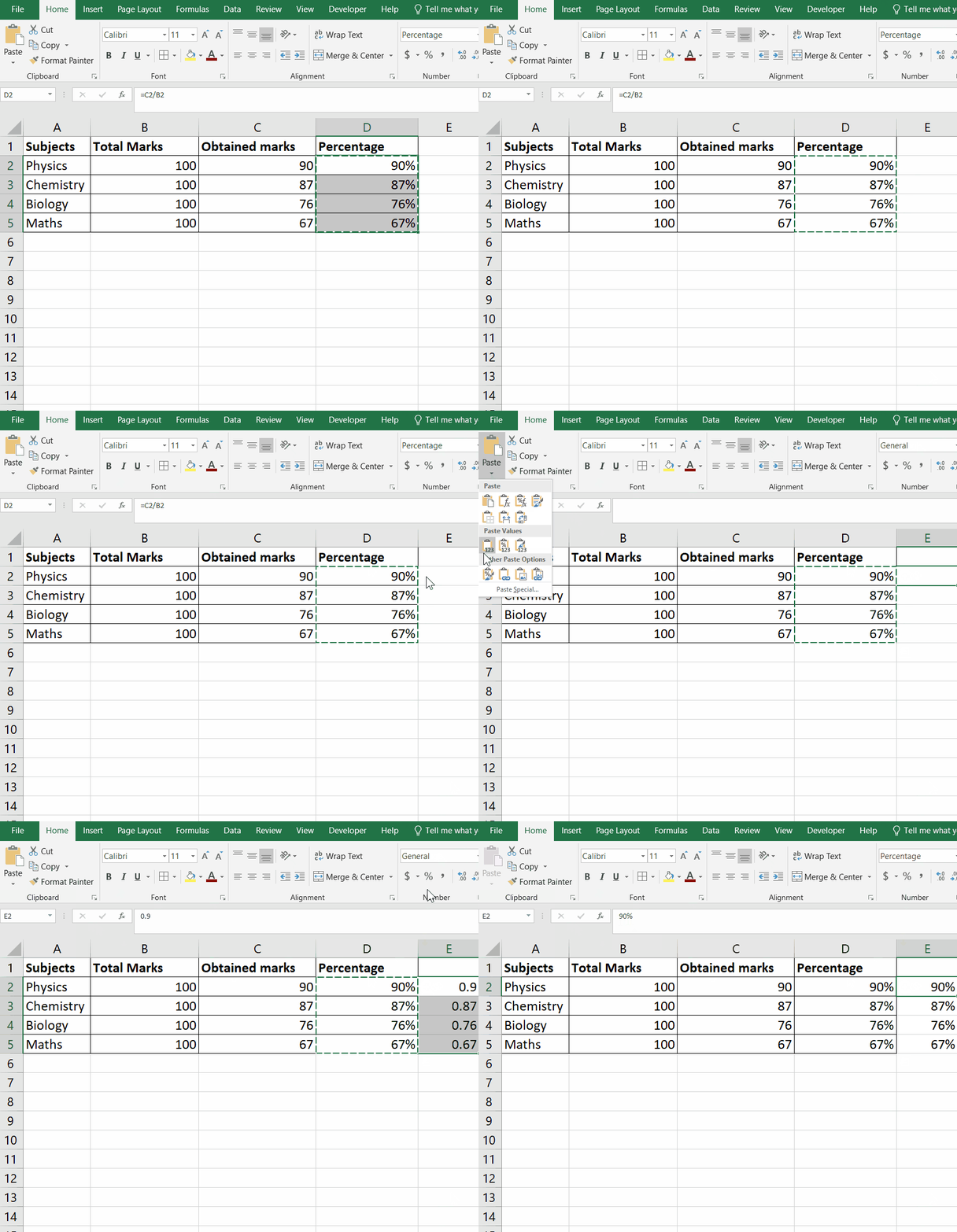
- Select the data range, in this case, we selected column D.
- Copy the data range or entire column, by right-clicking on it, a side menu will appear, click on Copy option.
- Or, click the keyboard shortcut Ctrl + C. All the selected data range or column will be copied to the clipboard.
- The formula bar shows the formula of percentage, as shown above.
Step 2 – Use Paste Special to convert the formula to text

- Go to the desired place as per your requirement and select the empty cell, where you wish to paste.
- In this case, we selected column E to paste and convert the formula into text.
- Go to the Home tab.
- In the menu bar, click on the Paste option.
- A drop-down menu will appear.
- Go to the Paste values, and select the first option Values(V).
- As soon as you press the enter key, all the data from column D will be pasted as text in column E.
- Press the percentage icon in the Numbers cluster, to convert the values into percentage.
- The formula bar will only show the numeric values in the newly pasted column as shown above.
Method 2 – Use paste special shortcut key
In this method, we will use MS Excel’s built-in tool to paste a special dialogue box. By using the shortcut key CTRL + ALT + V. The required steps are explained below;
Step 1 – Select the dataset with formulae and copy

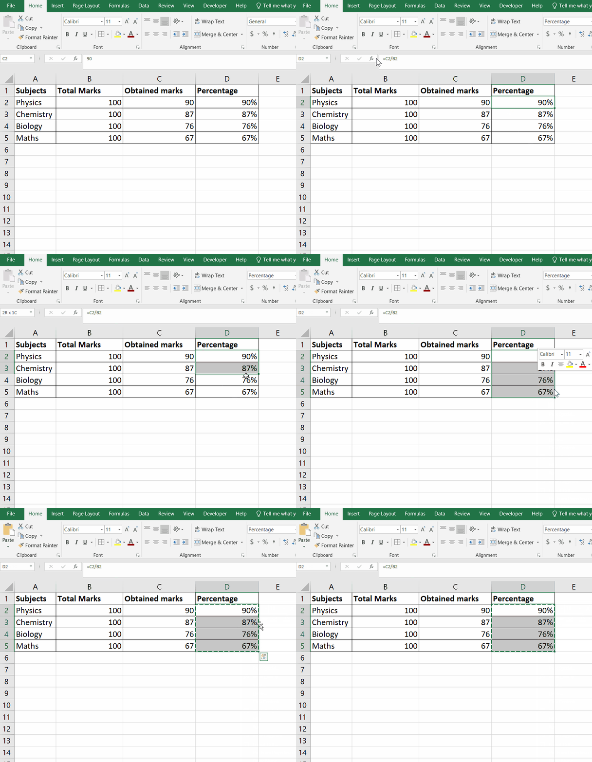
- Select the data range, in this case, we selected column D.
- Copy the data range or entire column, by right-clicking on it, a side menu will appear, click on Copy option.
- Or, click the keyboard shortcut Ctrl + C. All the selected data range or column will be copied to the clipboard.
- The formula bar shows the formula of percentage, as shown above.
Step 2 – Select the data range and paste special with shortcut

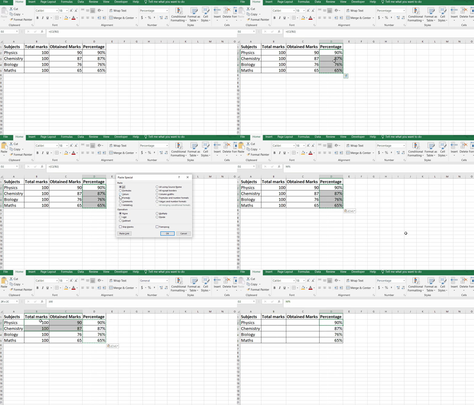
- Select the data range, in this case, we selected column D.
- Press the keyboard shortcut CTRL + ALT + V.
- A dialogue box will appear with the heading Paste special.
- Multiple options will be visible there. Click on the Values.
- Click on OK
- When you press the enter key, all the data from column D will be pasted as text in column D.
- The formula bar will only show the numeric values in the newly pasted column, as shown above.
Hence, by using the above two methods we can easily convert the formula into text. No error appeared even after deleting the source columns.


