
How to convert a pivot table to a regular table in Excel
 By
SpreadCheaters
By
SpreadCheaters
You can watch a video tutorial here.
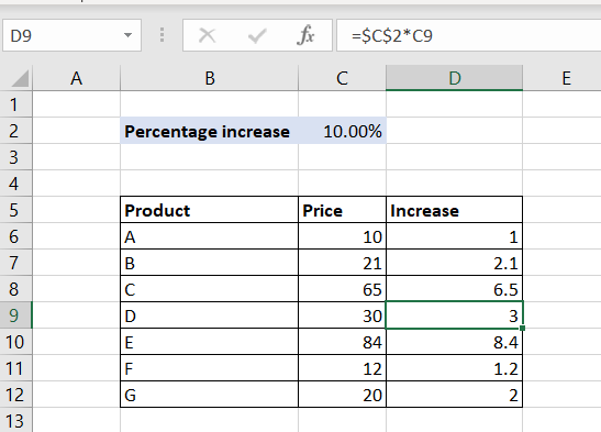
Pivot tables are one of the most useful tools in Excel for summarizing and analyzing data. Pivot tables are built off a table or a dataset and can summarize rows or columns. When you use a pivot table to summarize data you may need to convert it to a regular table so that it is no longer linked to the underlying data. You can then distribute it or use it to prepare a report.
Step 1 – Display in tabular form
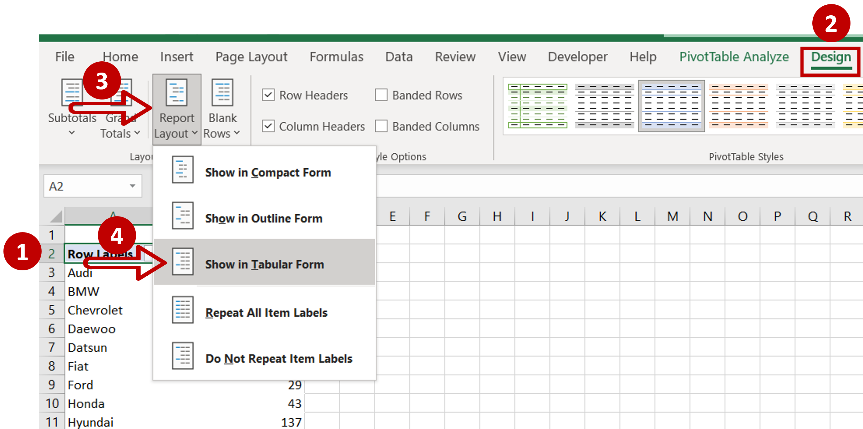
– Select any cell in the pivot table
– Go to Design > Layout
– Expand the Report Layout dropdown
– Click on the Show in Tabular Form option
– The field name is displayed
Step 2 – Copy the table
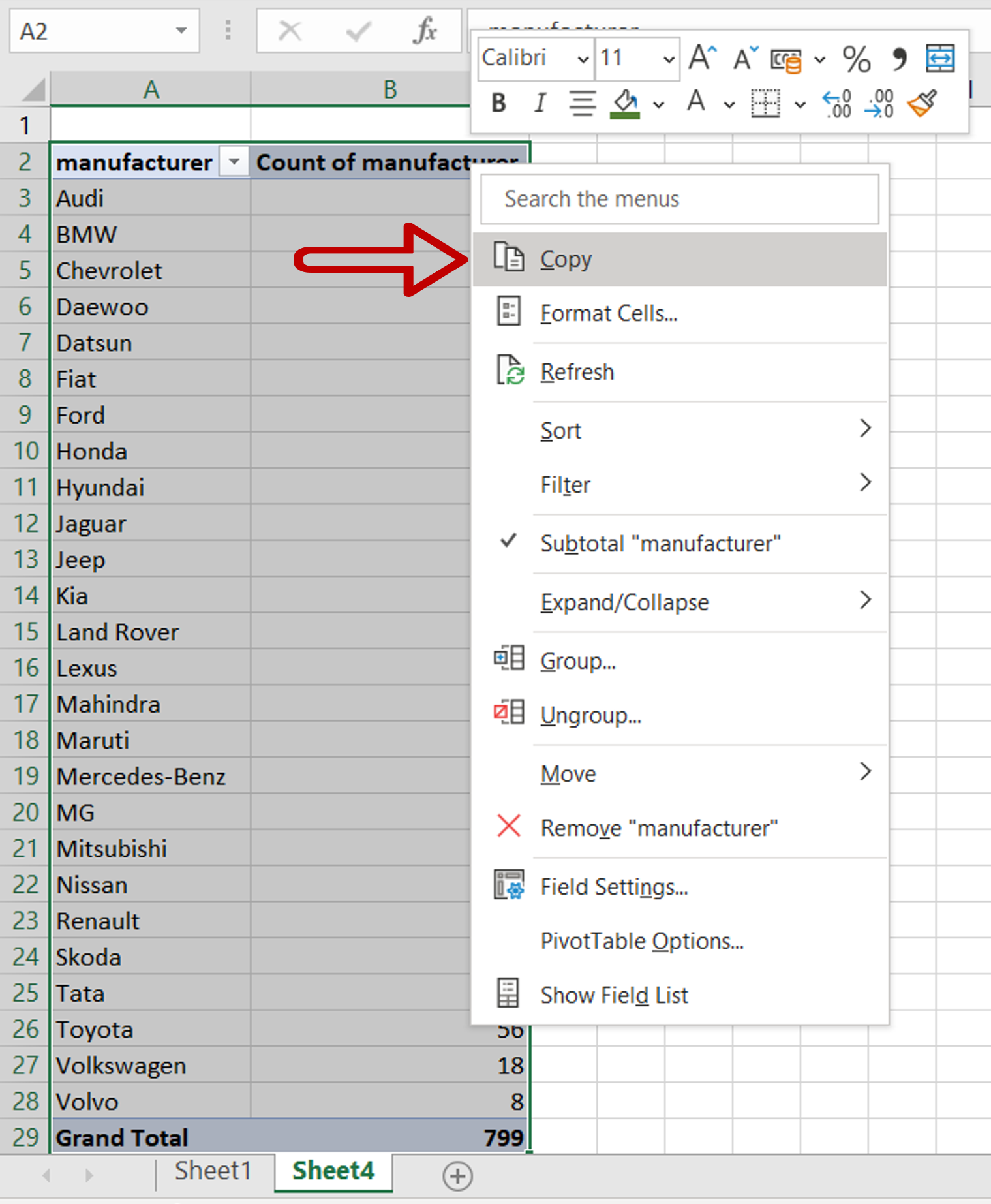
– Select the table and press Ctrl+C or right-click and select Copy from the context menu
Step 3 – Open the Paste Special window
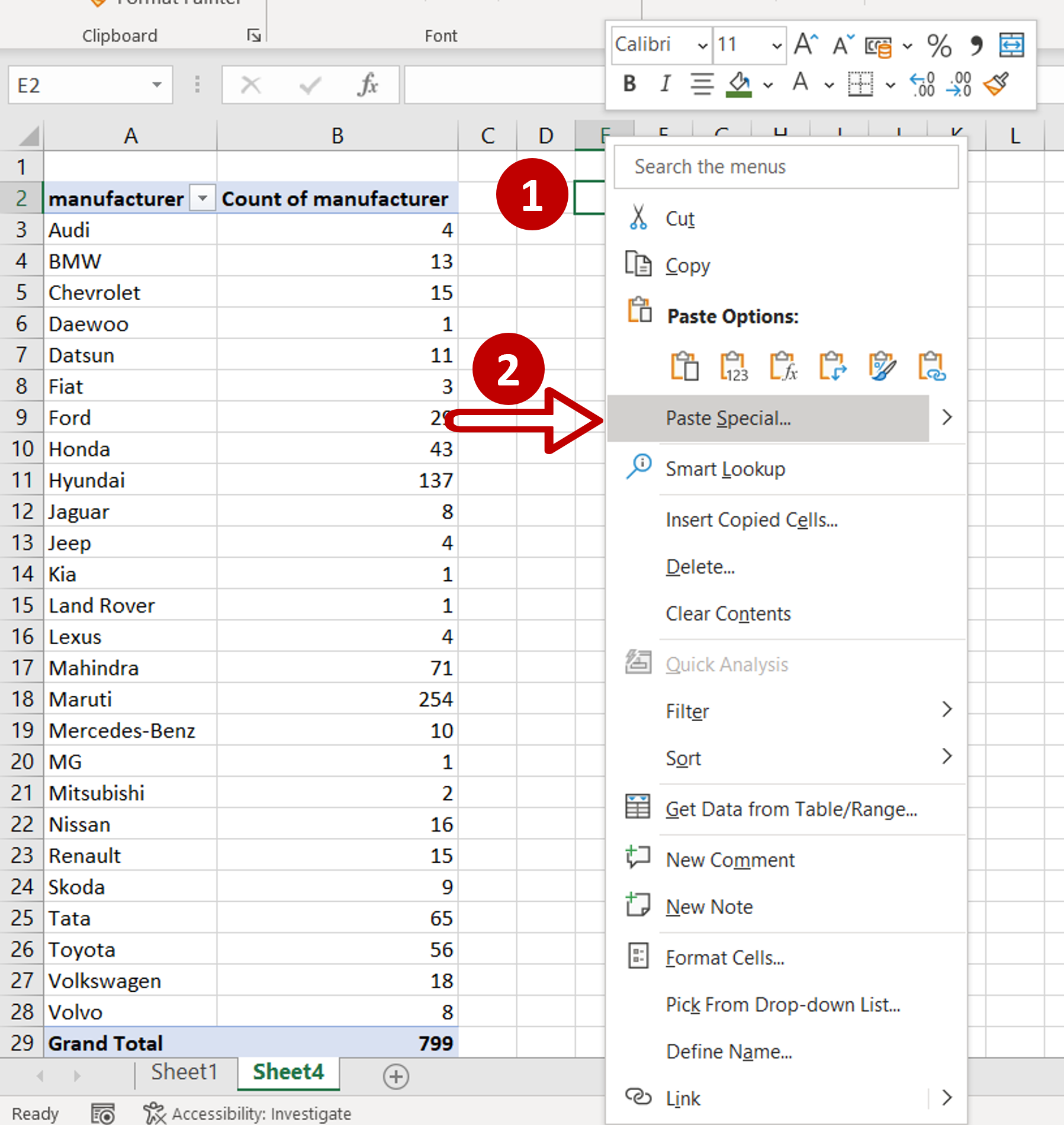
– Select the destination for the table
– Open the Paste Special window by right-clicking and selecting Paste Special from the context menu
OR
Go to Home > Clipboard > Paste > Paste Special
OR
Press Alt+E+S
Step 4 – Paste the table
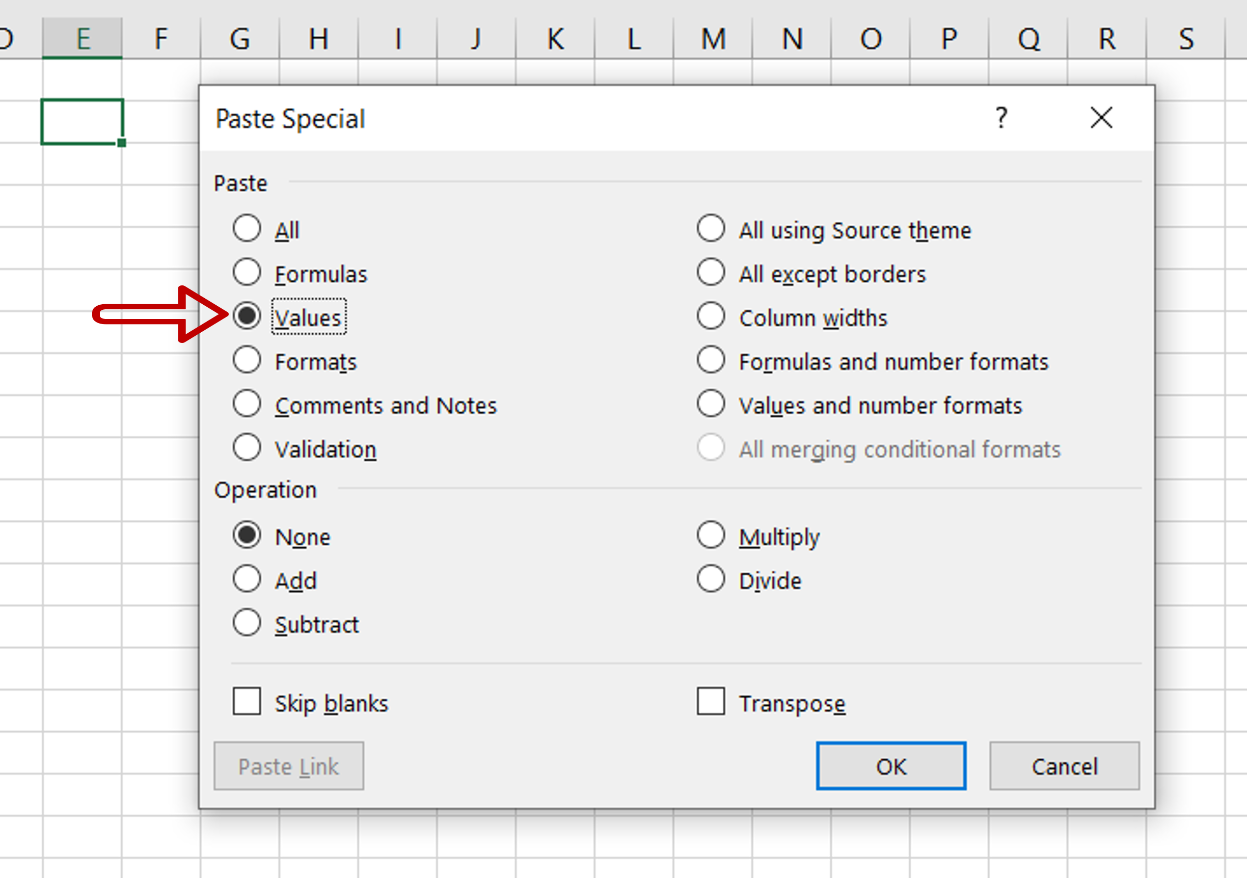
– Select Values
– Click OK
Step 5 – Check the result
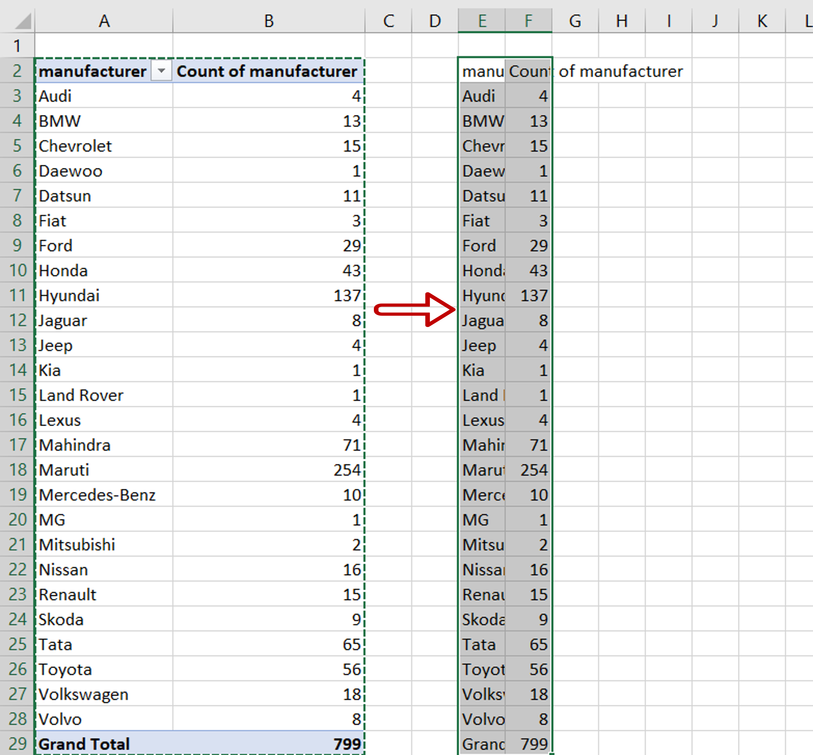
– The data is pasted as a regular table


