How to convert 8-digit number to date in Excel
Converting 8-digit numbers to date format in Excel is important because it allows you to work with dates in a more meaningful way. The 8-digit numbers in Excel represent dates in the format of YYYYMMDD. While this format might be useful for some purposes, it can be difficult to read and understand for many people. By converting these numbers to a date format, you can easily perform calculations, analyze trends, and sort data based on date.
For example, if you have a list of sales data with dates represented as 8-digit numbers, you can convert those numbers to a date format to analyze sales trends over time. Once the data is in date format, you can easily sort it chronologically, calculate monthly or quarterly sales totals, and create charts and graphs to visualize trends.
Excel doesn’t provide a straightaway function to perform this task. Therefore, we’ll have to use a customized solution based on various functions. We will use a combination of TEXT, DATE, LEFT, RIGHT, and MID functions.
Explanation of the functions to be used:
The TEXT function in Excel is used to convert a numeric value or date to a text string in a specific format. The syntax for the =TEXT function is as follows:
TEXT(value,format_text)
value: The numeric value or date that you want to convert to text.
format_text: The format that you want to apply to the value.
The DATE function is used to create a date from the year, month, and day components. The basic syntax of the DATE function is explained below;
DATE(year, month, day)
where:
year is the year component of the date, expressed as a four-digit number.
month is the month component of the date, expressed as a number between 1 and 12.
day is the day component of the date, expressed as a number between 1 and 31.
The LEFT function returns a specified number of characters from the beginning of a string. The syntax is as follows:
LEFT(text, num_chars)
text is the string from which you want to extract characters.
num_chars is the number of characters you want to extract from the left of the string.
The MID function returns a specified number of characters from a string, starting from a specified position. The syntax is as follows:
MID(text, start_num, num_chars)
text is the string from which you want to extract characters.
start_num is the position in the string where you want to start extracting characters.
num_chars is the number of characters you want to extract.
The RIGHT function returns a specified number of characters from the end of a string. The syntax is as follows:
RIGHT(text, num_chars)
text is the string from which you want to extract characters.
num_chars is the number of characters you want to extract from the right of the string.
The necessary steps are explained as follows;

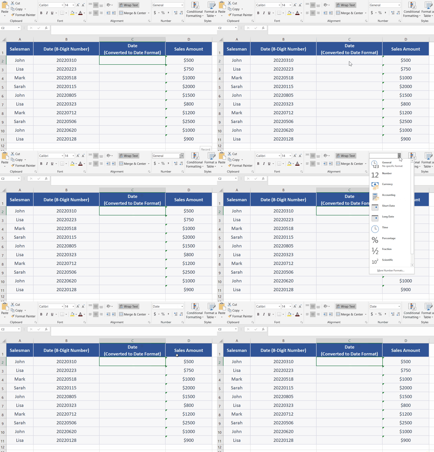
Step 1 – Select the desired cell and change the number format

– Select the cell where you want to display the date. In this case, we selected cell C2.
– Click on the “Number Format” dropdown menu in the “Home” tab of the Excel ribbon.
– Select “Short Date” from the list of formats. As shown above;
Step 2 – Change the date format

– Press a keyboard shortcut CTRL + 1.
– Click Date in the category.
– Select the suitable date format in the type segment i.e. [DD/MM/YYYY] etc.
– Click OK. As shown above;
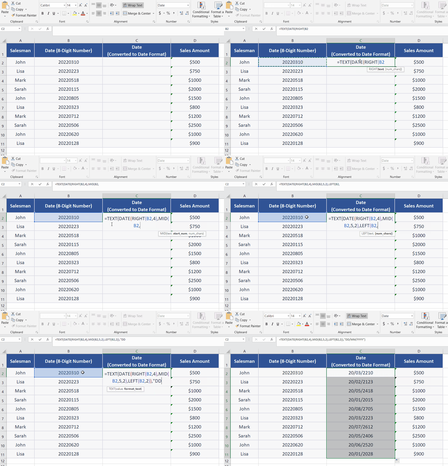
Step 3 – Apply the formula

Click on the cell where you wish to convert the 8-number digit into a date.
In this case, we selected cell B2.
In this case, we are using this formula =TEXT(DATE(RIGHT(B2,4), MID(B2,5,2), LEFT(B2,2)), “MM/DD/YYYY”).
This formula takes the 8-digit number in cell B2 and converts it to a date and text, using the DATE and TEXT functions.
As soon as you press the enter key, it will convert the numeric values into dates. As shown above;


