
How to compare two Excel files for duplicates
 By
SpreadCheaters
By
SpreadCheaters
Page last updated:
17/11/2022 |
Next review date:
17/11/2024
You can watch a video tutorial here.
Comparing two files for duplicates is an operation you will frequently need to do when working with datasets. This happens especially when you are combining data from multiple sources and need to identify duplicates or matches. In Excel, there are 2 ways of doing this:
- VLOOKUP() function: this searches for a value in the left-most column of a range, and returns the value in the column specified from the row of the match in the range.
- Syntax: VLOOKUP(lookup_value, table_array, col_index_num, range_lookup)
- lookup_value: the cell reference of the first value in the key column from Table 1 (Name)
- table_array: the range of Table 2 which is made constant with the addition of dollar signs ($)
- col_index_num: the number of the column in Table 2 that has to be retrieved (1 i.e. the Name)
- range_lookup: TRUE will return an approximate match, FALSE will return an exact match
- Syntax: VLOOKUP(lookup_value, table_array, col_index_num, range_lookup)
In this example, we will use VLOOKUP() to find values from the first file that match those in the second file.
- Conditional formatting: this will highlight duplicate values in a range of data
Option 1 – Use VLOOKUP()
Step 1 – Start typing the formula
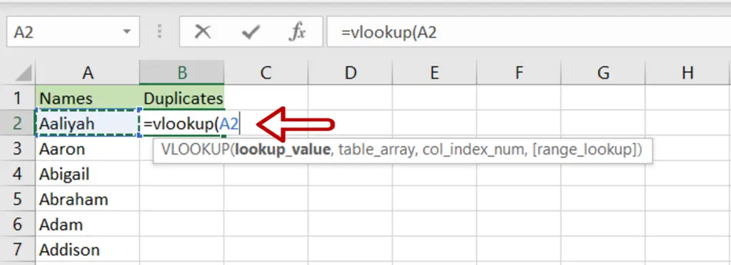
- Select the cell where the result is to appear
- Start typing the formula using cell references:
=VLOOKUP(Names,
Step 2 – Reference the second file
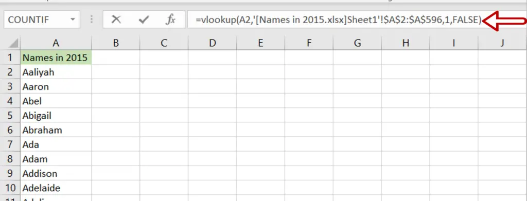
- Go to the second sheet and select the range of the column that is being compared
- The range will be added to the formula with the file and sheet name
- The range reference will automatically be made constant
- Complete the formula”
= VLOOKUP(Names, range in the second file, 1, FALSE)
- The col_index_num is set to 1 because there is only one column
- Press Enter
Step 3 – Enhance the formula to handle errors i.e. missing values
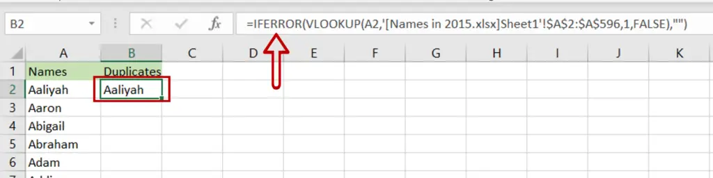
- If the lookup function cannot find a match in the second file i.e. ‘Names in 2015’, an error message will be returned – #N/A
- Change the formula to display an empty cell if a match cannot be found:
= IFERROR(<vlookup formula>,””)
Step 4 – Copy the formula
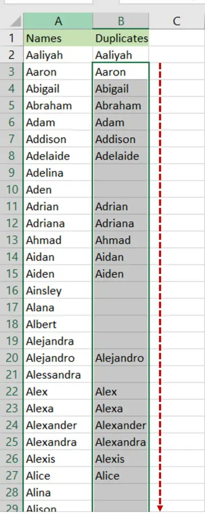
- Select the cell with the formula and press Ctrl+C
- Press Ctrl+Shift+Down arrow to go to the end of the column
- Press Enter
- The formula will be copied to the rest of the column
Step 5 – Check the result
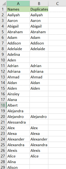
- The ‘Duplicates’ column has the list of duplicates between the two files
Option 2 – Use conditional formatting
Step 1 – Copy the column to be compared from the second file
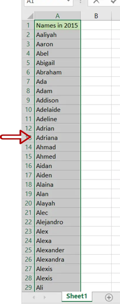
- Select the column to be compared in the second file
- Press Ctrl+C
Step 2 – Paste the column
- Go to the first file
- Select the column next to the column being compared
- Press Ctrl+V
Step 3 – Open the Duplicate Values box
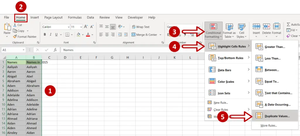
- Select both columns
- Go to Home > Style > Conditional Formatting
- From Highlight Cells Rules select Duplicate Values
Step 4 – Choose the format
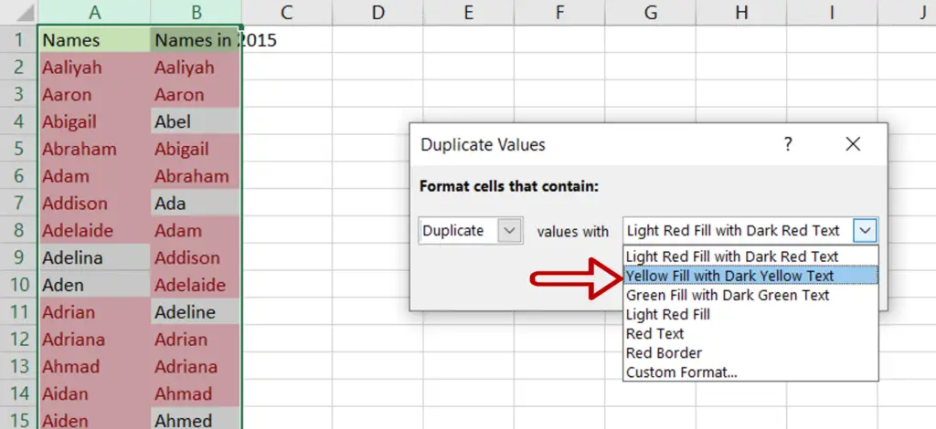
- Select the Yellow Fill with Dark Yellow Text option
- Click OK
Step 5 – Check the result
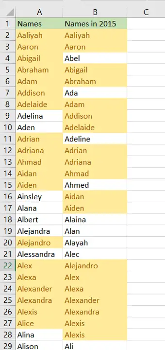
- Values that are duplicated in the list are highlighted in the given format


