How to compare two columns in Microsoft Excel and remove the duplicates 

Comparing two columns in Excel and removing duplicate values is a useful task when working with large datasets. By comparing two columns, you can quickly identify matching or non-matching values in different columns of data. Removing duplicate values from these columns helps to eliminate redundancy and ensure data accuracy. 

In this tutorial, we will learn how to compare two columns in Microsoft Excel and remove the duplicates. To compare two columns and remove duplicates we can use the Conditional Formatting feature or we can use a combination of multiple formulas i.e. IF, VLOOKUP, etc.

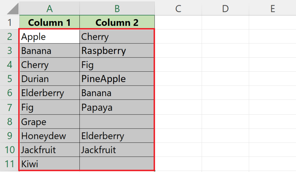
We currently have a dataset with two columns, each containing a list of fruits, but there are some fruits that appear in both columns. We aim to eliminate the duplicates from the first column so that both columns contain only unique fruits.

Method  1: Using IF, ISNA, and VLOOKUP Function

This method will use a combination of VLOOKUP, ISNA, and IF functions to create a customized formula to find out duplicates. We’ll check all the entries from the first column one by one and check if there exists any duplicate of these entries. If a duplicate is found then it will be labeled as Duplicate otherwise Unique.

Step 1 – Create a Helper Column

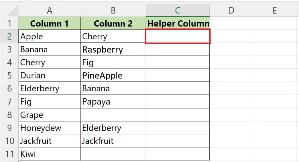
• Create a helper column.
• We will use the helper column to filter out the Unique values and will label them as Unique or Duplicate in this column.

Step 2 – Select a Blank Cell and Place an Equals Sign

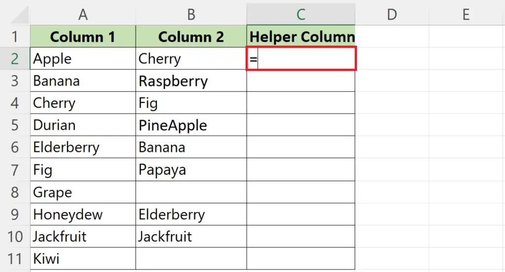
• Select a blank cell in the helper column.
• Place an Equals sign in the blank cell.

Step 3 – Enter the IF and ISNA Function

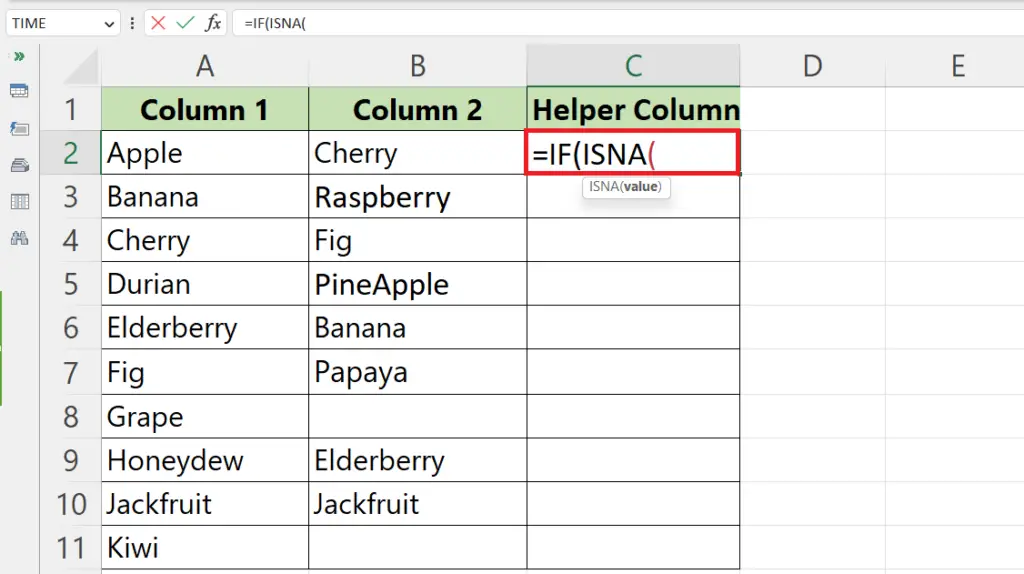
• Enter the IF function next to the Equals sign.
• Enter the ISNA function as the logical test(first argument) of the IF function.

Step 4 – Enter the VLOOKUP Function

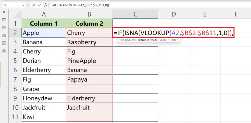
• Enter the VLOOKUP function as an argument of the ISNA function.
• The syntax of the VLOOKUP function is as follows:

             IF(ISNA(VLOOKUP(A2,$B$2:$B$11,1, False)),

• Where A2 is the cell with the lookup_value and $B$2:$B$11 is the lookup_array.
• The third argument 1 represents the column’s index in the lookup_array which is 1.

Step 5 – Enter the “Value_if_true” 

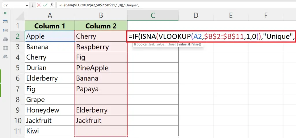
• Enter the “Value_if_true” i.e. unique.

            IF(ISNA(VLOOKUP(A2,$B$2:$B$11, 1, FALSE)), “Unique”,

Step 6 – Enter the “Value_if_false” 

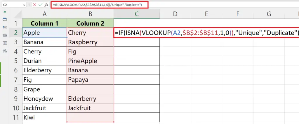
• Enter the “Value_if_false” i.e. Duplicates.

            IF(ISNA(VLOOKUP(A2,$B$2:$B$11, 1, False)), “Unique”,  “Duplicates”)

Step 7 – Press the Enter Key

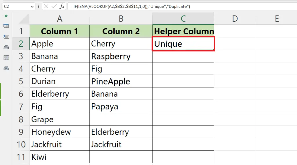
• Press the Enter key to get the results.

Step 8 – Use Autofill to Mark All Values as Duplicate or Unique 

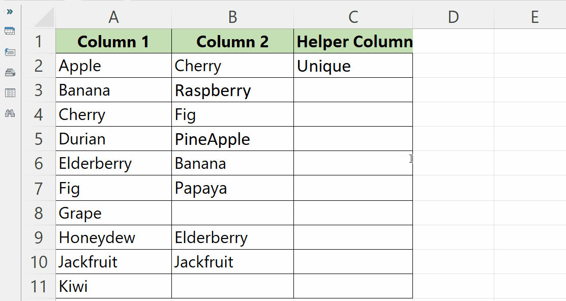
• Use Aufofill to mark the values as Duplicate or Unique.

Step 9 – Select the Helper Column and Apply the Filter 

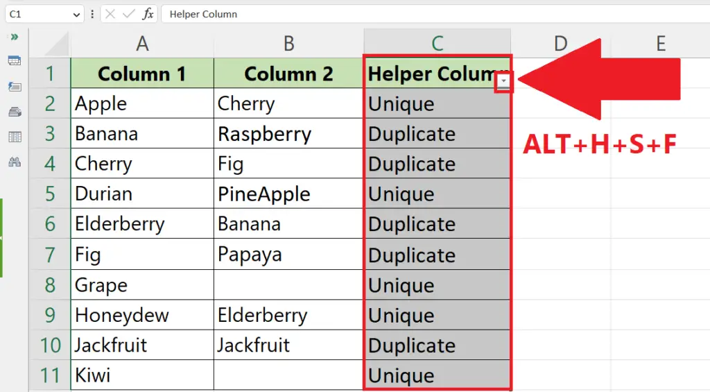
• Select the helper column.
• Apply the Filter on the column by pressing ALT+H+S+F.
• The filter drop-down arrow will appear, next to the header of the helper column.

Step 10 – Filter for “Duplicates”

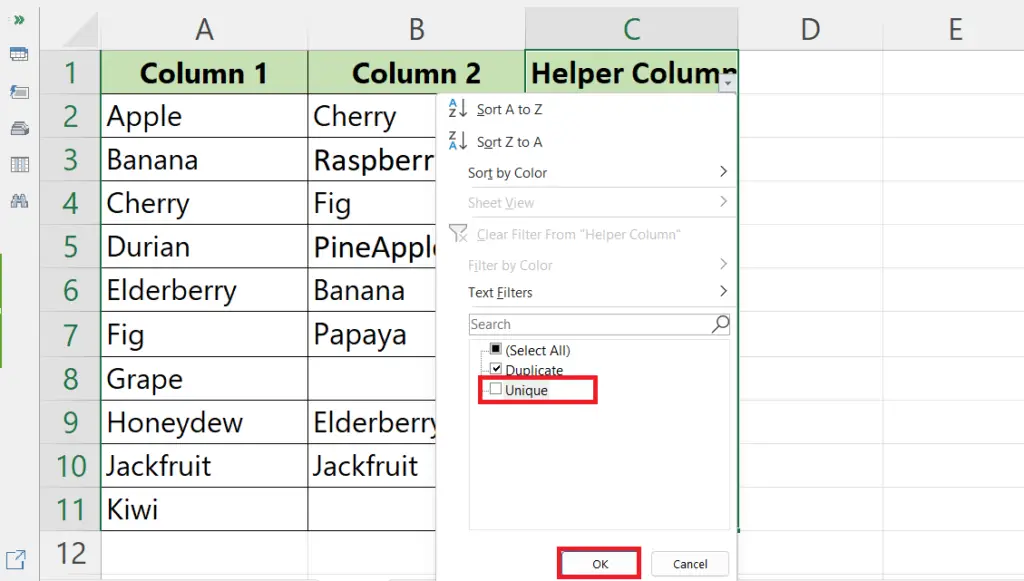
• Click on the Filter arrow.
• Uncheck the box with “Unique”.
• Click on OK.
• Only the cells containing “Duplicates” would be visible.

Step 11 – Now Delete the Column Containing the Lookup_Values for the VLOOKUP Function

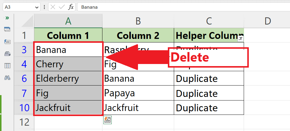
• Select the first column of the range, i.e. the column that contained the lookup values for the VLOOKUP function.
• Delete the column.

Step 12 – Disable the Filter

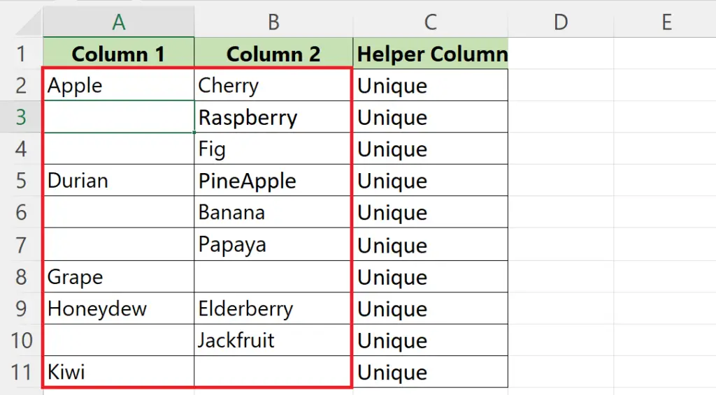
• Disable the Filter.
• For this, press ALT+H+S+F or we can disable the filter from the Home tab.
• Only Unique values would now be visible in both columns and the duplicates would be removed.

Method 2: Using Conditional Formatting

Step 1 – Select Both the Columns

• Select both columns to be compared.

Step 2 – Click on the Conditional Formatting Button

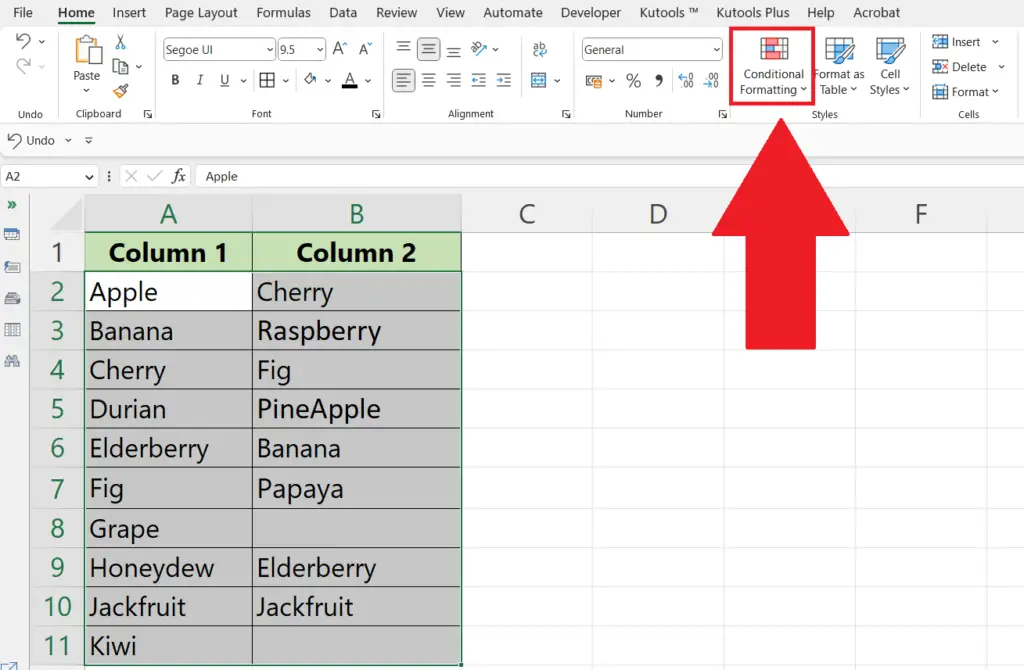
• Click on the Conditional formatting button in the Styles section of the Home tab.

Step 3 – Click on the “Highlight Cell Rules” and Select “Duplicate Values”

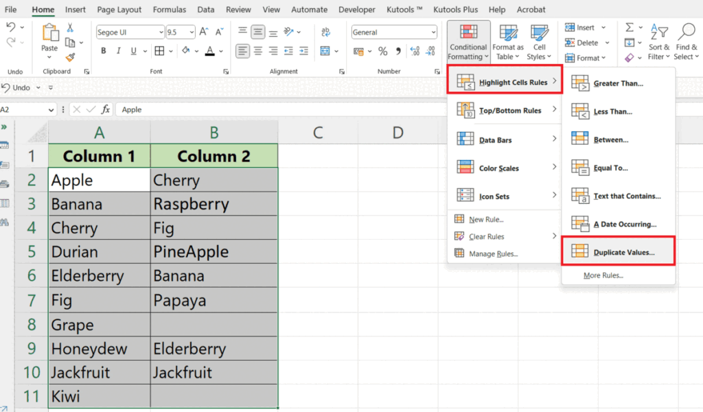
• Click on the “Highlight Cell Rules”.
• Select “Duplicate Values”.
• All the duplicate values will be highlighted.
• Click on OK in the dialog box that appears.

Step 4 – Select a Column and Apply the Filter 

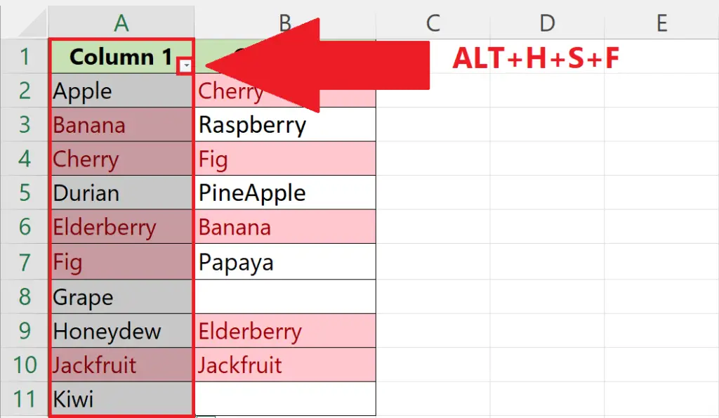
• Select the column from which you want to remove the duplicate values.
• Apply the Filter on the column by pressing ALT+H+S+F.
• The filter drop-down arrow will appear, next to the header of the helper column.

Step 5 – Filter By Color

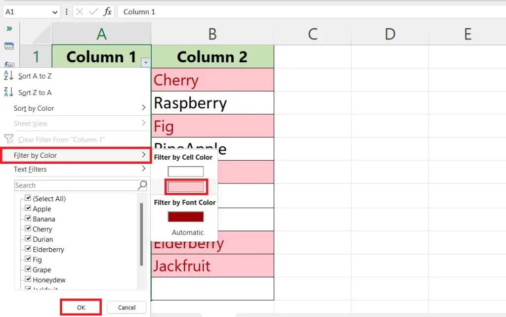
• Click on the Filter arrow.
• Click on the FIlter by color.
• Select the color.
• Click on OK in the drop-down menu.

Step 6 – Now Delete the Visible i.e. Highlighted Cells from the Column

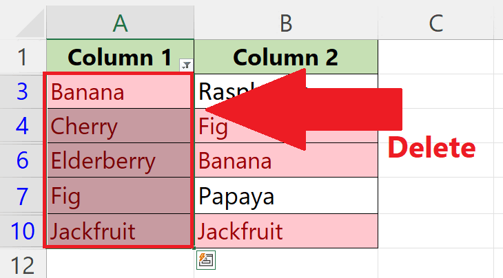
• Delete any one of the columns i.e. the columns from which you want to delete the duplicate values.

Step 7 – Disable the Filter

• Disable the Filter.
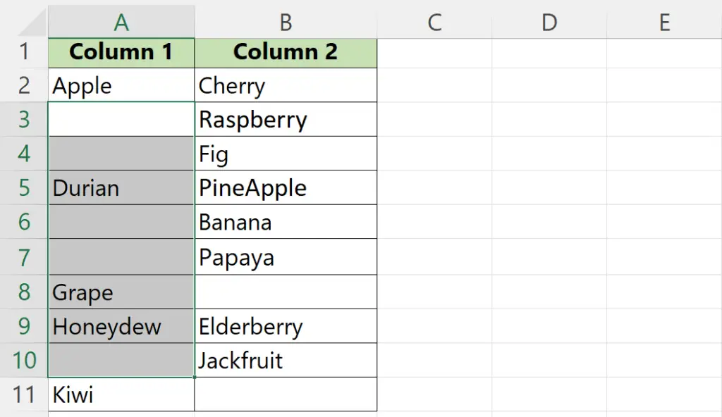
• For this, press ALT+H+S+F or we can disable the filter from the Home tab.
• Only Unique values would now be visible in both columns and the duplicates would be removed.

Explanation of the formula used in Method 1:

IF(ISNA(VLOOKUP(A2,$B$2:$B$11, 1, False)), “Unique”,  “Duplicates”)

The above formula is used to identify duplicate values in column A by checking if the corresponding value in column B is the same as the value in column A. Here is a breakdown of how the formula works:

The VLOOKUP function searches for the value in cell A2 in the range B2:B11 (i.e., column B).

The fourth argument of the VLOOKUP function is set to False, which means an exact match is required. If the VLOOKUP function finds a match, it returns the corresponding value from column B. If it doesn’t find a match, it returns an error value.

The ISNA function checks if the result of the VLOOKUP function is an error value. If it is, this means there is no corresponding value in column B, so the value in column A is unique.

If the result of the ISNA function is TRUE, the formula returns the text “Unique”. If the result of the ISNA function is FALSE, this means there is a corresponding value in column B, so the value in column A is a “Duplicate”.  

If the result of the ISNA function is FALSE, the formula returns the text “Duplicates”.

In summary, the formula checks if each value in column A has a corresponding value in column B. If it does, it marks it as a duplicate. If it doesn’t, it marks it as unique.