How to compare two columns in Excel for missing values

Comparing two columns for missing values in Excel means identifying the cells in one column that do not have corresponding values in another column. This is commonly used when dealing with large sets of data where there are multiple columns with related information. It helps to  easily identify which cells are empty or contains different values, allowing you to clean up the data or reconcile any discrepancies.

In this tutorial, we will learn how to compare two columns in Excel for missing values. Multiple built-in functions in Microsoft Excel can be utilized while comparing two columns. These include the VLOOKUP, IF, ISNA, ISNUMBER, and Match functions. Also, we can use Conditional formatting to compare two columns for the missing values.

Let’s say we have two sets of data – a column showing all the students in a class i.e. Columns A and a column showing the students who are present on a given day i.e. Column F. To mark the attendance of the students, we need to compare the two columns and identify which students are present and which are absent.

Method 1: Comparing Two Columns Using IF, ISNA, and the VLOOKUP Functions

Step 1 – Select a Blank Cell and Place an Equals Sign

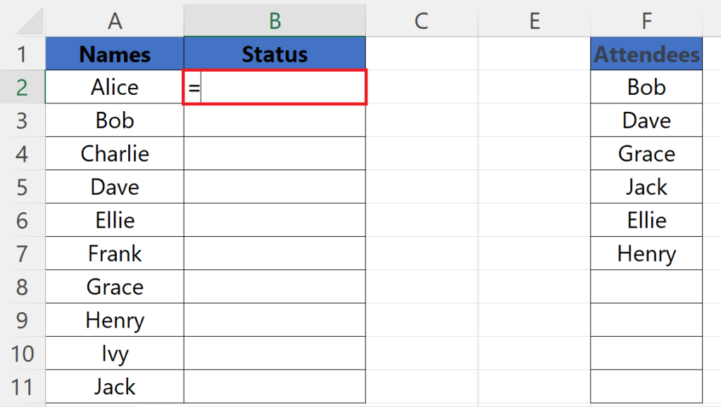
• Select a blank cell.
• Place an Equals sign in the blank cell.

Step 2 – Enter the IF and ISNA Function

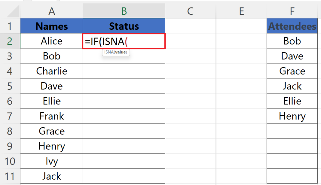
• Enter the IF function next to the Equals sign.
• Enter the ISNA function as the logical test(first argument) of the IF function.

Step 3 – Enter the VLOOKUP Function

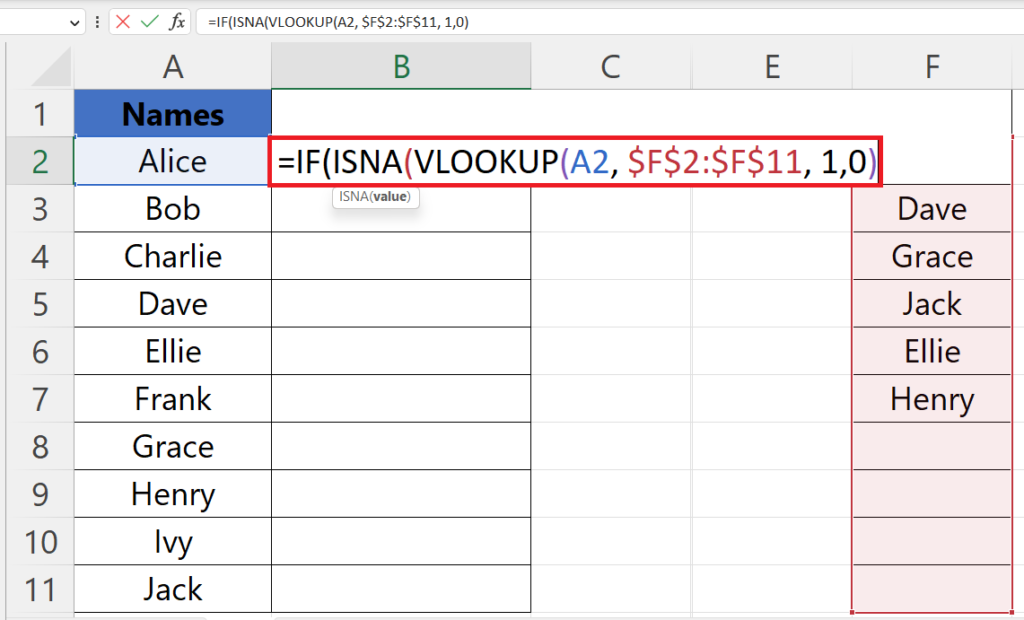
• Enter the VLOOKUP function as an argument of the ISNA function.
• The syntax of the VLOOKUP function is:

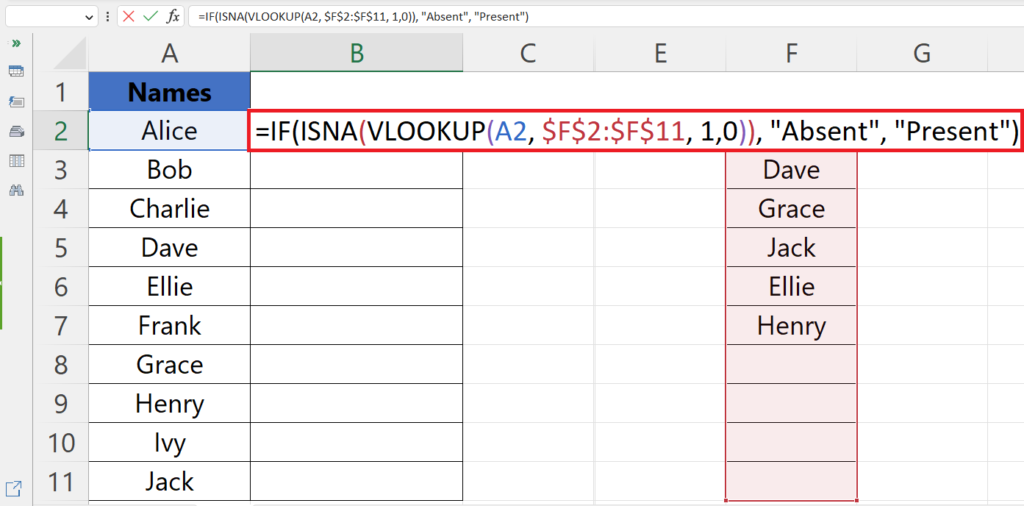
             IF(ISNA(VLOOKUP(A2,$F$2:$F$11,1, False)),

• Where A2 is the cell with the lookup_value and $F$2:$F$11 is the lookup_array.
• The third argument 1 represents the column’s index in the lookup_array which is 1.

Step 4 – Enter the “Value_if_true” 

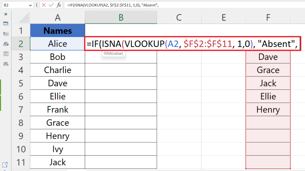
• Enter the “Value_if_true” i.e. Absent.

            IF(ISNA(VLOOKUP(A2,$F$2:$F$11, 1, FALSE)), “Absent”,

Step 5 – Enter the “Value_if_false” 

• Enter the “Value_if_false” i.e. Present.

            IF(ISNA(VLOOKUP(A2,$F$2:$F$11, 1, False)), “Absent”, ”Present”)

Step 6 – Press the Enter Key

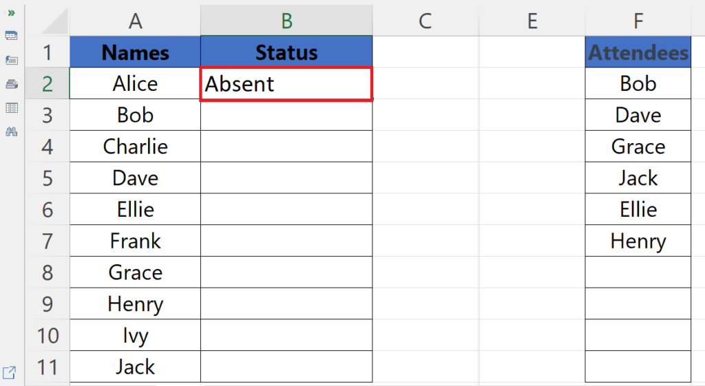
• Press the Enter key to get the results.

Step 7 – Use Autofill to Mark the Attendance For Each Student

• Use Aufofill to mark the attendance for Each student.

Breakdown of the formula used:

IF(ISNA(VLOOKUP(A2,$F$2:$F$11, 1, False)), “Absent”, ”Present”)

The formula is used to check if the value in cell A2 exists in the range F2:F11, and return “Absent” if it does not exist, and “Present” if it does. Here’s how the formula works:

The VLOOKUP function searches for the value in cell A2 in the range F2:F11. The fourth argument of the VLOOKUP function is set to False, which means an exact match is required. If the VLOOKUP function finds a match, it returns the corresponding value from column F. If it doesn’t find a match, it returns an error value.

The ISNA function checks if the result of the VLOOKUP function is an error value. If it is, this means there is no corresponding value in the range, and the formula returns the text “Absent”.

If the result of the ISNA function is FALSE, this means there is a corresponding value in the range, and the formula returns the text “Present”.

In summary, the formula checks if the value in cell A2 exists in the range F2:F11. If it does, it marks it as “Present”. If it doesn’t, it marks it as “Absent”. This formula can be copied down to check for the presence or absence of other values in column A in the same range.

Method 2: Using the MATCH Function and ISNUMBER Functions

Step 1 – Select a Blank Cell and Place an Equals Sign

• Select a blank cell.
• Place an Equals sign in the blank cell.

Step 2 – Enter the ISNUMBER and MATCH Function

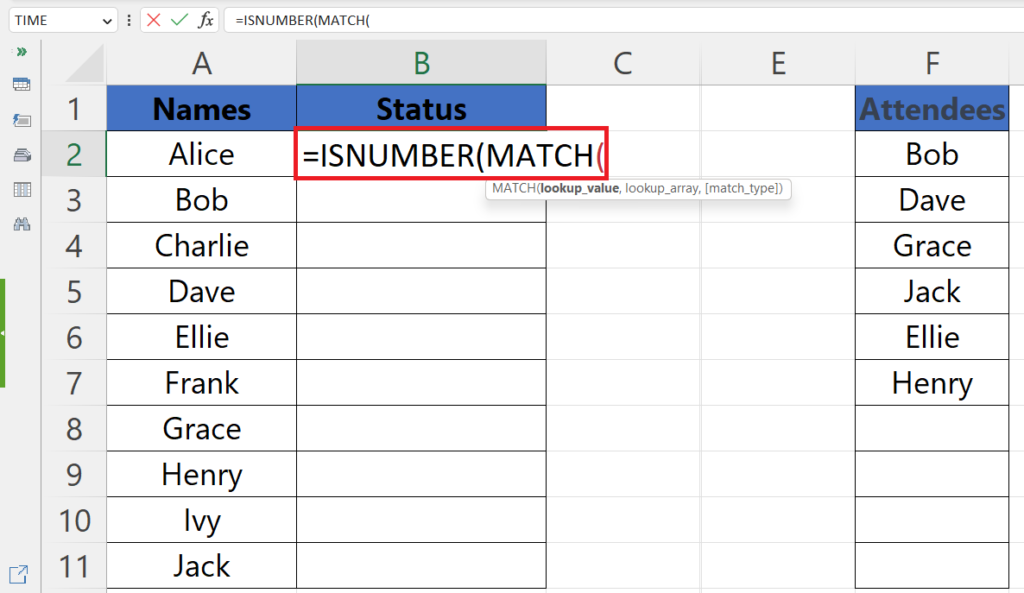
• Enter the ISNUMBER function next to the Equals sign.
• MATCH function as the logical test for the ISNUMBER function.
• The ISNUMBER function returns TRUE if the value returned is a number, else it returns false.

Step 3 – Enter the Arguments For the Match Function

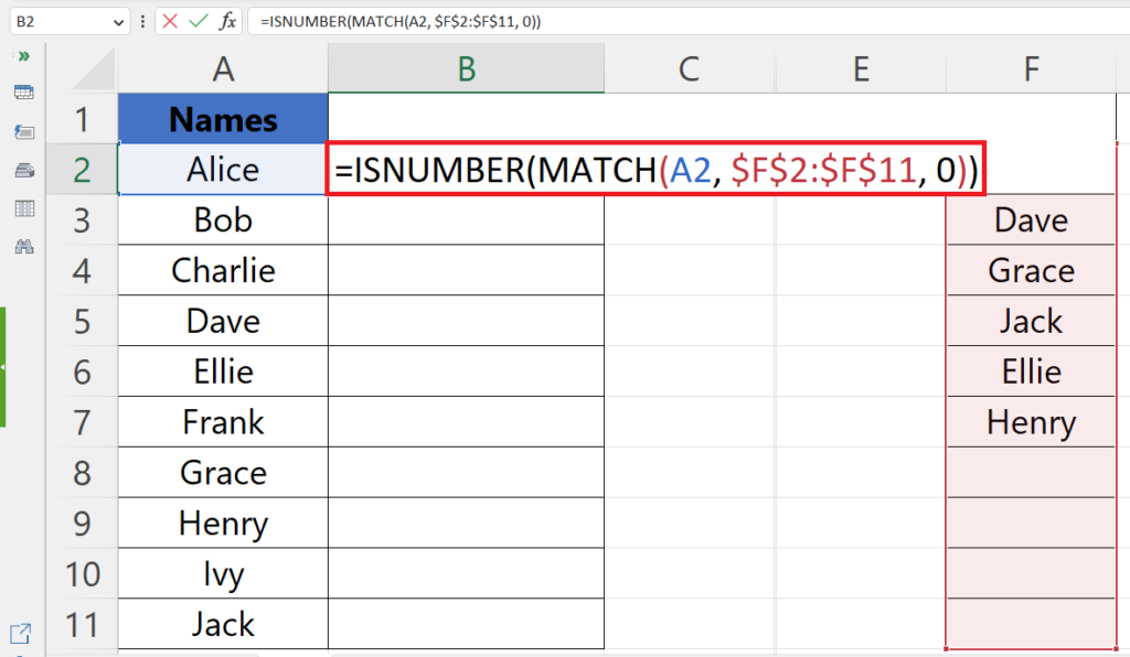
• Enter the arguments for the MATCH function.
• The syntax of the MATCH function is:

            ISNUMBER(MATCH(A2, $F$2:$F$11, 0 )

• Where A2 is the cell with the lookup_value and $F$2:$F$11 is the lookup_array.
• The third argument 0 represents the match type.

Step 4 – Press the Enter Key

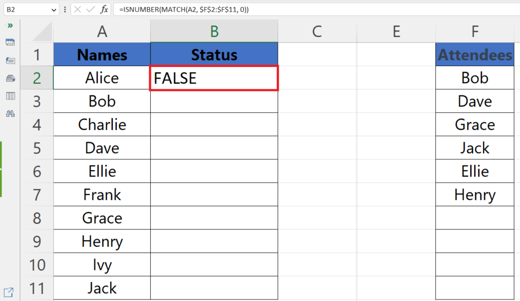
• Press the Enter key to get the result.
• The value formulae will return “TRUE” if present and “False” is absent.

Step 5 – Nest the Formula in the IF Function

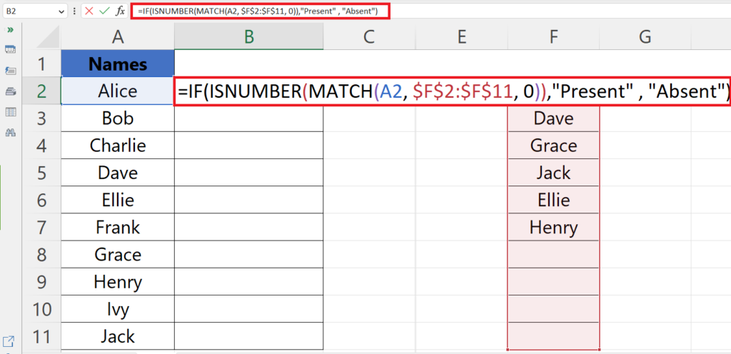
• Nest the complete formulae in the IF function to return desired values i.e.
  “Present” and “Absent”.
• The syntax will become:

            IF(ISNUMBER(MATCH(A2, $F$2:$F$11, 0 ), “Present”, “Absent”)

• Press the Enter key now to get the desired results.

Step 6 – Use Autofill to Mark the Attendance For Each Student

• Use Aufofill to mark the attendance for Each student.

Breakdown of the formula used:

IF(ISNUMBER(MATCH(A2, $F$2:$F$11, 0)), “Present”, “Absent”)

The formula provided checks whether the value in cell A2 is present in the range F2:F11. 

It does so by using the MATCH function to search for an exact match of the value in A2 within the range. If the MATCH function returns a number, the value is found in the range and the ISNUMBER function will evaluate to TRUE. The formula will therefore return “Present”. 

If the MATCH function returns an error value, the value is not found in the range and the ISNUMBER function will evaluate to FALSE. In this case, the formula will return “Absent”. 

Method 3: Using the Conditional Formatting

Step 1 – Select the Range

• Select the range containing both columns to be compared.

Step 2 – Click on the Conditional Formatting Button and Click on New Rule

• Click on the Conditional Formatting button in the Home tab.
• Click on the New Rule option.

Step 3 – Select “Format only unique or duplicate values” Option

• Select the “Format only unique or duplicate values” option in the Select a Rule Type section.

Step 4 – Select “Unique” in the “Format all” List

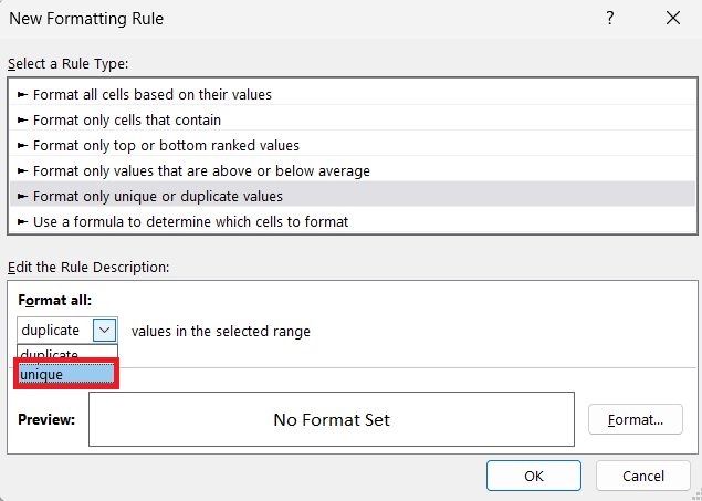
• Select the “Unique” option in the “Format all” drop-down list.

Step 5 – Click on the Format Button and Select Formatting Manually

• Click on the Format button in the dialog box.
• Select a Format i.e. a fill color to highlight the missing values.

Step 6 – Click on OK 

• Click on OK in the Format Cells dialog box.
• Then, click on OK in the New Formatting Rule dialog box.
• The missing values will be highlighted.