How to compare data from two worksheets in Excel

When you are working with small data files in Excel and you are asked to compare data within two different versions of the same file then it can be an easy task if you have sharp eyes and the number of data points in the files are only a few. 

However, if you have to do the same job when the files contain large data sets then trying to do this manually can be very tedious and time taking. If you know how to use some specific functions which will be tailored to your particular requirement, then Excel will come to your rescue and help you to accomplish this complicated task.

There are two methods to compare the data from two worksheets present in the same Excel file.

• Compare data by using an IF formula
• Compare data by using conditional formatting with custom formula

Let’s explore both options one by one through this example data which is not very large but for the sake of explaining the process of comparing the data sets it will work just fine.

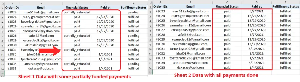
 In these data sets we can see that the status of the payments is different in both sheets. The sheet 2 is updated with payments statuses as paid and sheet1 shows them partially_refunded. Imagine having thousands of such entries in both sheets then you won’t be able to do this manually. Therefore, let’s use the power of Excel to find out the differences in both sheets. We’ll achieve this by both methods which were mentioned earlier.

Method 1: Compare Data using Excel’s IF formula

To use the effect of the formula first we need to view the sheets side by side to see them and compare them through a formula. So follow along these steps to create side by side views of the sheets and then to compare them.

Step 1 – Open both sheets of the same file in two windows

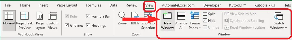
• Open the Excel file, locate the View tab from the list of tabs.
• In the Window group, click the New Window button as shown in the figure above.
• This will open the same excel file in a new window.

Step 2 – Enable Side by Side View

• To view the sheets side by side, press the Side by Side button in the Window Group.
• Select Sheet1 in the first window and Sheet2 in the second window.

Step 3 – Implement the IF formula to compare data on a new sheet

• We will have to add a new empty sheet to the same workbook to create a difference report for Sheet1 and Sheet2.
• We will use a simple formula which is;

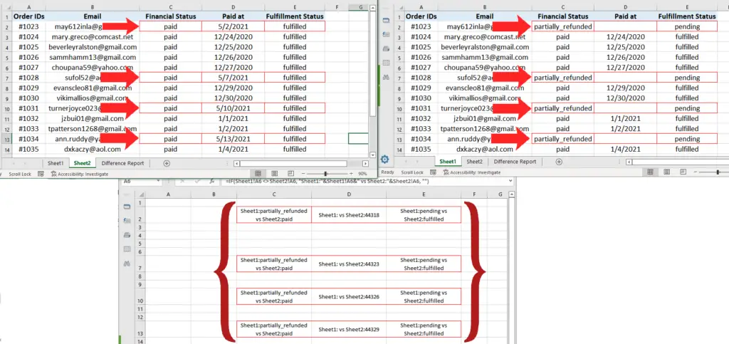
=IF(Sheet1!A1 <> Sheet2!A1, “Sheet1:”&Sheet1!A1&” vs Sheet2:”&Sheet2!A1, “”)

This formula will compare the first Cells of both sheets and in case of difference it will display the contents of both cells from both sheets opposite to each other to show the actual difference.

• In this formula we have used relative cell references so these will change according to the cell positions when we drag this formula to the desired range and will produce the results as shown above.

The difference report shown at the bottom of the above picture has those cells filled with values which were different in both sheets. So now we know which cells in both sheets are different from each other.

Method 2: Compare Data using conditional formatting

We can use conditional formatting to identify the differences in both sheets of the same workbook as well. This method is slightly different from the first one but more effective because it will highlight all the differences in both sheets one by one. We’ll apply conditional formatting in both sheets one after the other. So let’s follow the below mentioned steps to achieve this.

Step 1 – Open and View the sheets side by side

• To do this repeat steps 1 & 2 from the first method again.

Step 2 – Select the whole data range in the sheet

• In the sheet where you want to apply the conditional formatting, select the first cell of the data range and then press “CTRL + SHIFT + END” keys to select the complete data range as shown above.

Step 3 – Locate Conditional Formatting in Styles group on Home tab

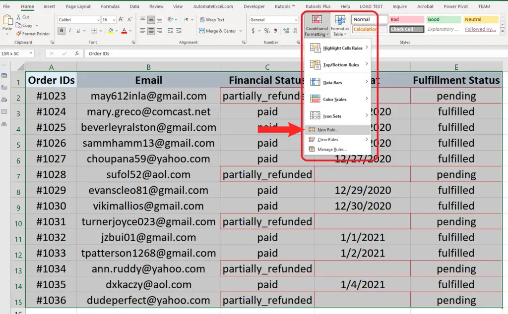
• After selecting the data range, on the Home tab go to Styles group and click on Conditional Formatting and then select New Rule as shown above.

Step 4 – Use Conditional Formatting to create New Rule

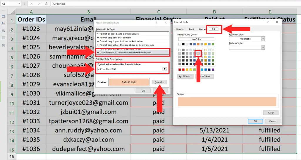
• When you click on New Rule, A window New Formatting Rule will appear and it will ask you to select a rule type for conditional formatting.
• Select Use a formula to determine which cells to format and then create a new rule using the following simple formula;

=A1<>Sheet2!A1

This formula tells Excel to check if the value of cell A1 in the current sheet is not equal to A1 of sheet2 then apply the desired format to the cells.

• After writing the formula, click on the Format button. A new dialog Format Cells will appear, select Fill in the new dialog box and then select any colour to fill the background of the cell meeting the formula condition as shown above.

Step 5 – Implement Conditional Formatting to highlight differences

• After selecting the colour to fill in, press the OK button in the Format Cells dialog box.
• You will come back to the New Formatting Rule window. Press the OK button and all the cells which are different in sheet1 from sheet2 will be highlighted with the colour of your choice as shown above;
• In the animation below, you will see that I had already marked the different cells with a red outline. This was done just to give an idea that if conditional formatting works fine then these are the cells which should be highlighted.
• To implement the same thing in Sheet2, repeat all steps as before. However, for sheet 2 use this formula instead;

=A1<>Sheet1!A1

So this is how you can compare the worksheets present in the same Excel file using the conditional formatting’s custom formula option.