How to combine two rows in Excel

You can watch a video tutorial here.

Combining rows in Excel is most often used when formatting tables, to make the table more readable.  When a value is repeated multiple times across two rows, within the same column, it is better to combine the rows so that the value is displayed only once. If the rows to be merged are blank, then the solution is simple. If the rows contain data, then there are different solutions depending on whether all the data is to be retained or not. 

Option 1 – Only the data in the first row is to be retained

Step 1 – Select the rows 

• Select the rows to be combined

Step 2 – Navigate to the Merge menu

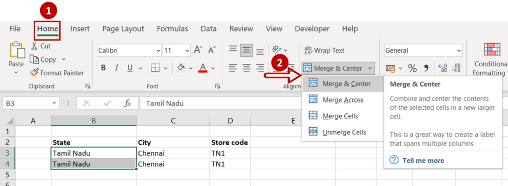
• Go to the Home menu
• Expand the Merge & Center option on the Alignment section

Step 3 – Merge the cells

• Select Merge & Center
  • With the Merge & Center option, the data from the top row is positioned at the bottom of the cell, in the center
  • With the Merge Cells option, the data from the top row is positioned at the bottom of the cell, aligned to the left
• A warning will be displayed
• Click OK

Option 2 – Data in both rows is to be retained

Step 1 – Open the clipboard

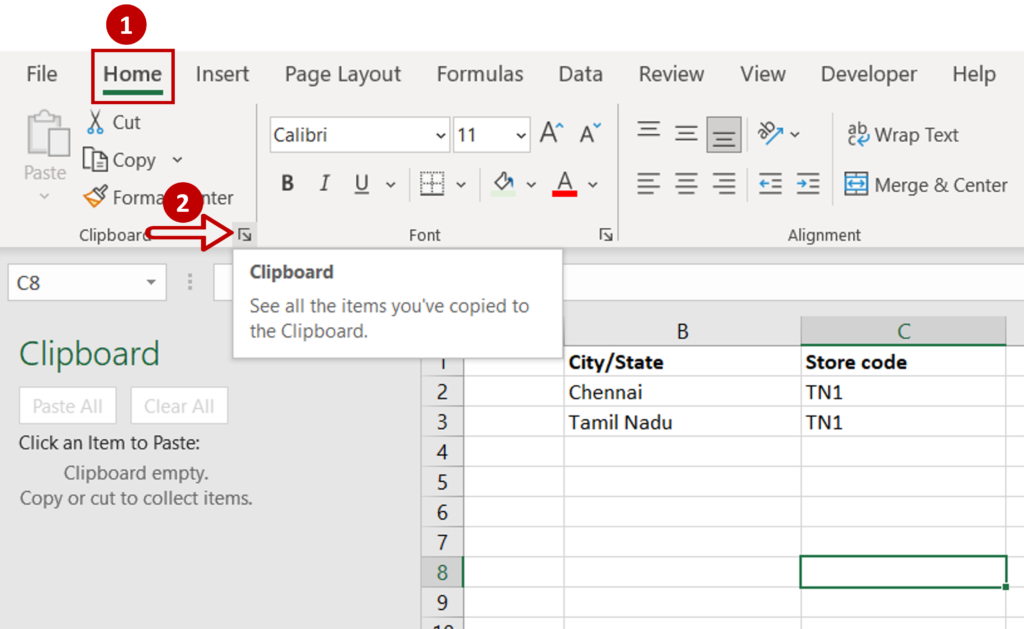
• Go to the Home menu
• Open the Clipboard

Step 2 – Copy the data

• Select the rows to be merged and click Ctrl+C
• The data will be copied onto the clipboard

Step 3 – Paste the data into the top cell

• Double-click on the top cell or place the cursor on the cell and click F2
• Delete the data in the cell
• Click on the item in the clipboard
• The data will be pasted into the cell
• Press Enter

Step 4 – Navigate to the Merge menu

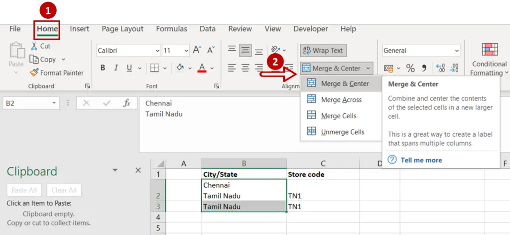
• Select the cells to be merged
• Got to Home > Alignment > Merge & Center

Step 5 – Merge the cells

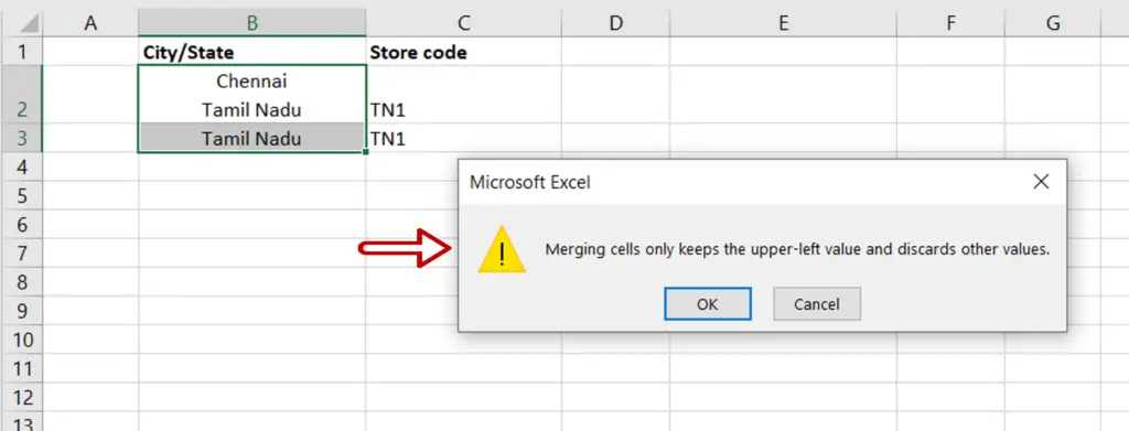
• Select Merge & Center
  • With the Merge & Center option, the data from the top row is positioned at the bottom of the cell, in the center
  • With the Merge Cells option, the data from the top row is positioned at the bottom of the cell, aligned to the left
• A warning will be displayed
• Click OK