
How to combine two pivot tables in Excel
 By
SpreadCheaters
By
SpreadCheaters
You can watch a video tutorial here.
Pivot tables are one of the most useful tools in Excel for summarizing and analyzing data. Pivot tables are built off a table or a dataset and can summarize rows or columns. You can create multiple pivot tables from an underlying data source, each presenting you with a different insight into the data. Having built multiple pivot tables, you may want to combine two of them into a single pivot table. Pivot tables can be combined only if they are built off the same data source and if they are grouped on a similar field. The data source can be a single dataset or a data model.
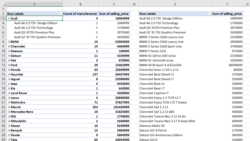
Step 1 – Analyze the pivot tables
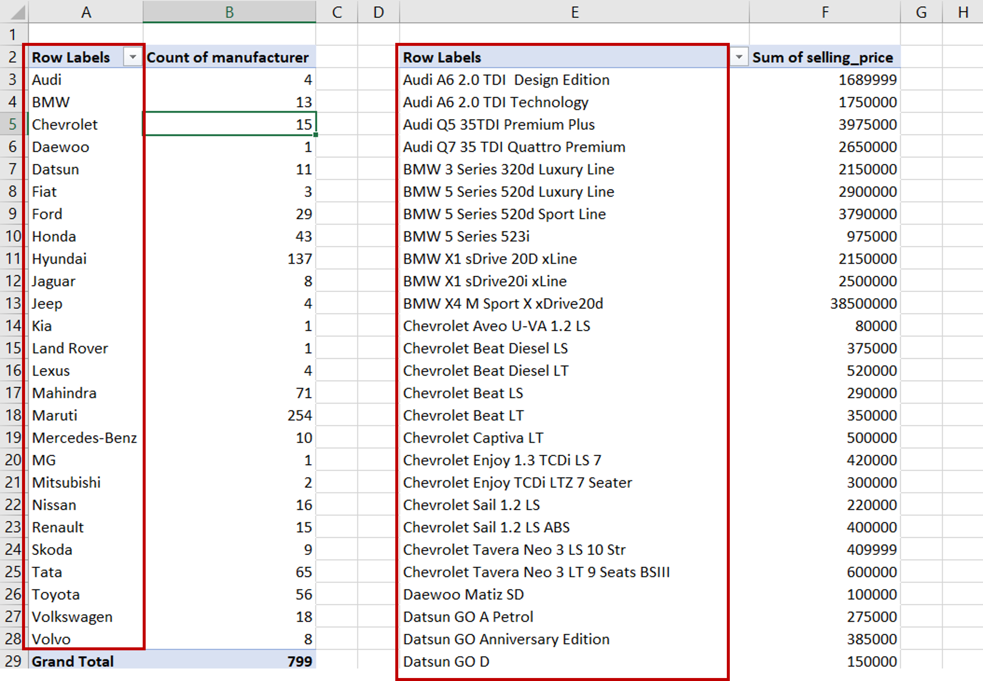
– Check that both the tables are grouped on a similar field
– The row labels in the second table are a sub-group of the row labels in the second table
– Both pivot tables have the same data source
Step 2 – Open the Field List
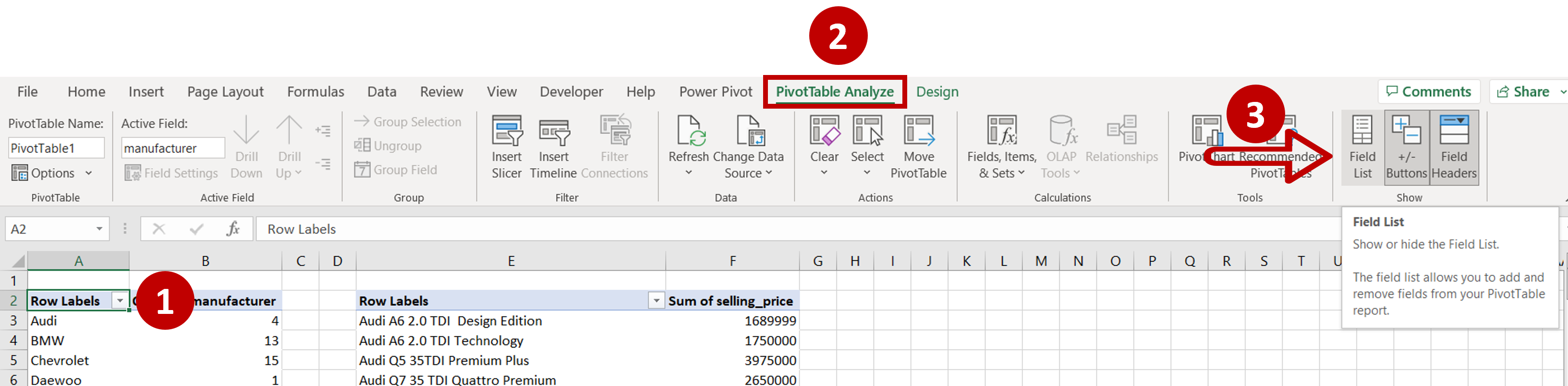
– Select any cell in the first pivot table
– Go to PivotTable Analyze > Show
– Click on the Field List button
Step 3 – Add the first field from the second pivot table
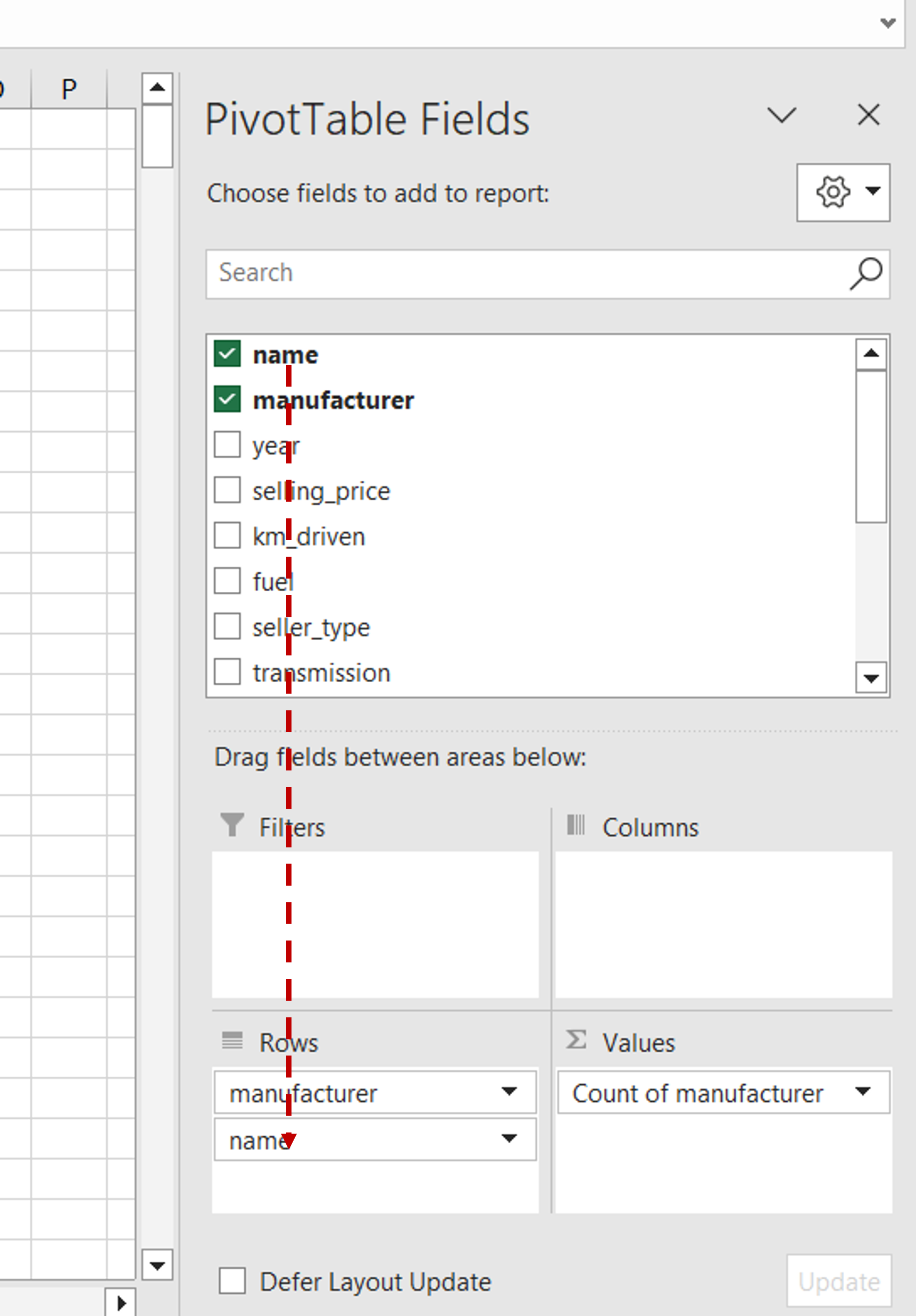
– Drag the ‘name’ field down to beneath the ‘manufacturer’ field under Rows
Step 4 – Add the second field
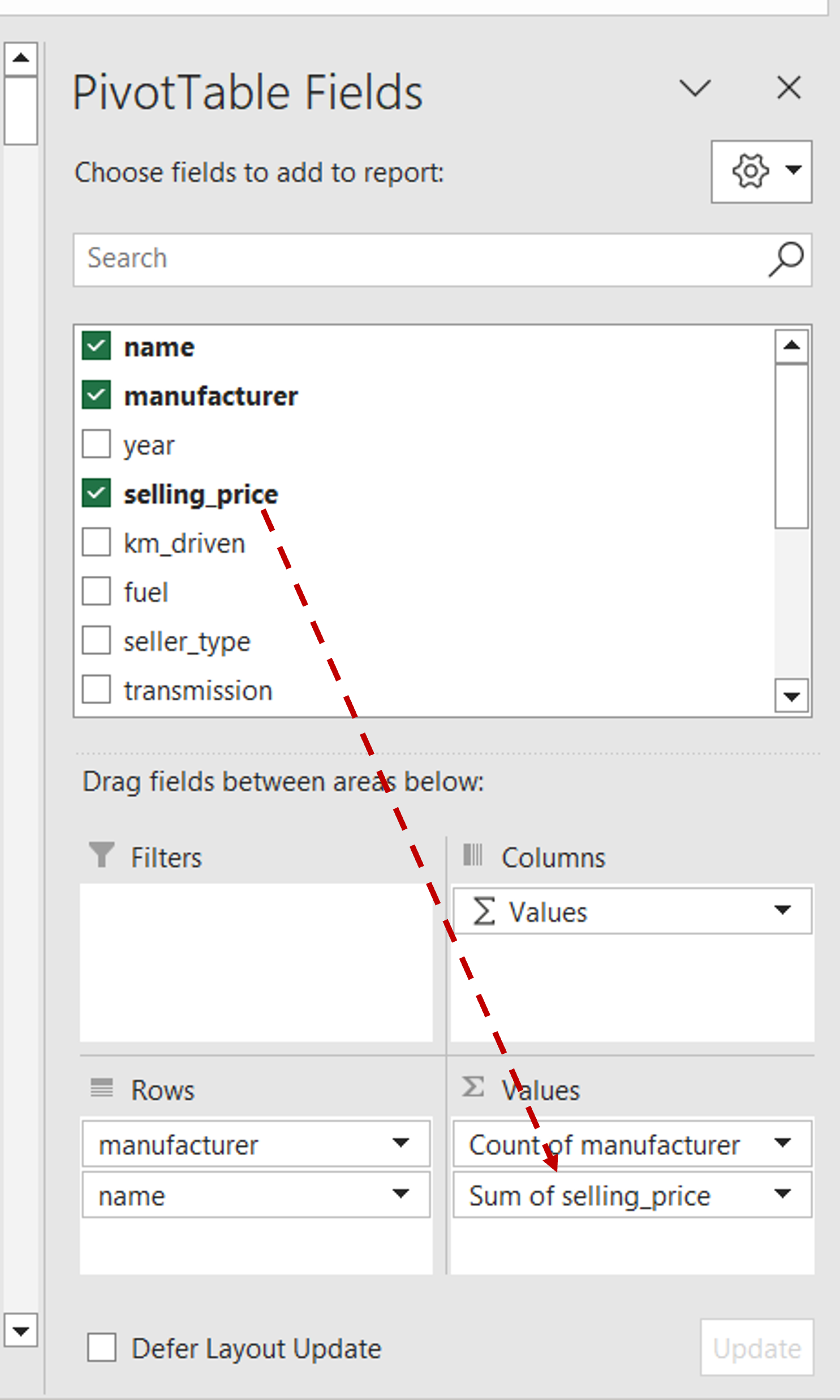
– Drag the ‘selling_price’ field to the Values section, under ‘Count of manufacturer’
– The ‘Sum’ aggregation function is automatically applied
Step 5 – Check the result
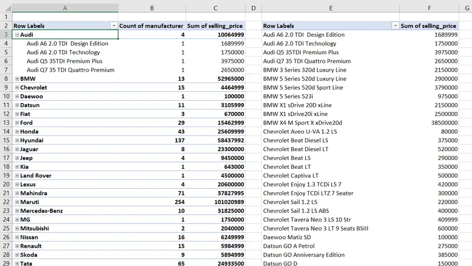
– The pivot tables are combined into a single pivot table
– Expand the group in the first pivot table to see the details
– The second pivot table can be deleted if it is not needed


