
How to combine two cells in Excel with a dash
 By
SpreadCheaters
By
SpreadCheaters
Combining two cells in Excel with a dash means merging the contents of two cells into a single cell, and separating them with a dash (-) symbol. Overall, combining two cells in Excel with a dash can make your data more organized and easier to understand, especially when you need to present the data to others.
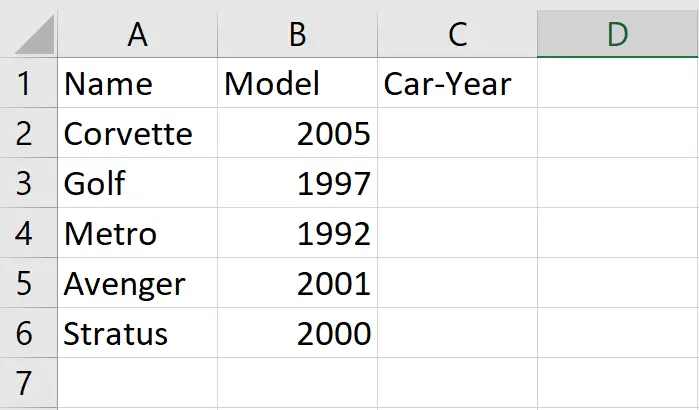
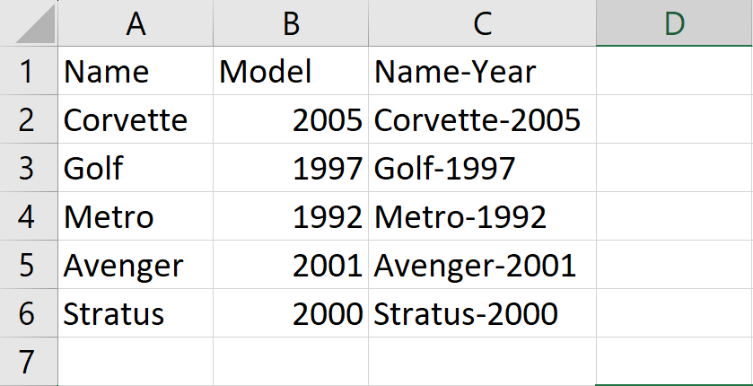
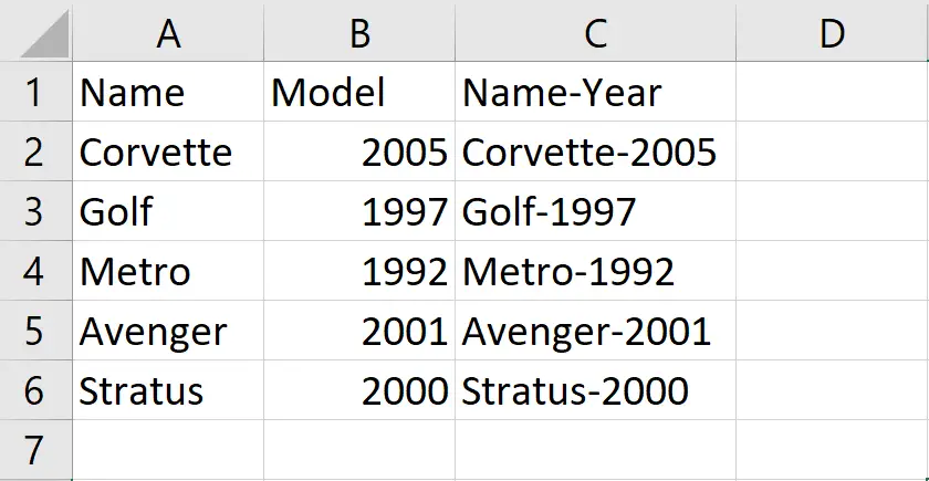
Our dataset includes car names and their corresponding models written in separate columns. We aim to merge them into a single column separated by a dash symbol. We can achieve this in three ways. The first method is to use the CONCATENATE function, the second is to use a formula, the third is to use the JOINTEXT function and the fourth is to use the CONCATENATE function.
Method 1: Combine cells separated with a dash using the CONCAT function
The CONCAT function in Excel is used to combine two or more text strings into a single cell or range. The function was introduced in Excel 2016 as an improvement over the older CONCATENATE function.
The syntax of the CONCAT function is as follows:
CONCAT(text1, [text2], [text3], …)
- text1: The first text string to concatenate. This argument is required.
- [text2], [text3], etc.: Additional text strings to concatenate. You can include up to 253 text arguments.
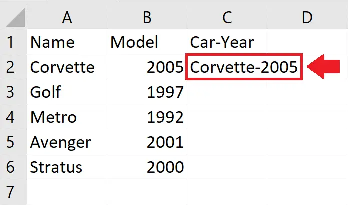
Step 1 – Select the cell

- Click on the cell where you want to combine the cells
Step 2 – Use the CONCAT Function
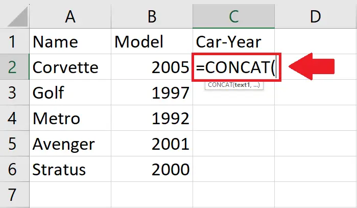
- After selecting the cel, use the CONCAT function by typing “=CONCAT(”
Step 3 – Type the Arguments of Function
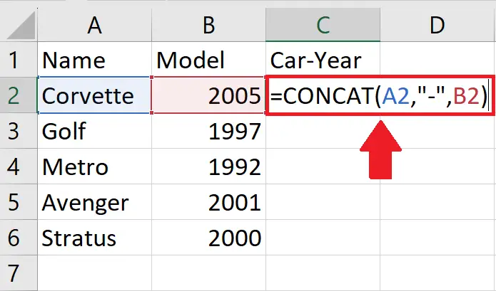
- After typing the CONCAT function, type the arguments as follows:
- Text 1: A2
- After text 1, type “-”
- Text 2: B2
- After typing the arguments, type a closing bracket “)”
Step 4 – Press the Enter key

- After typing the arguments, press the Enter key to get the required result
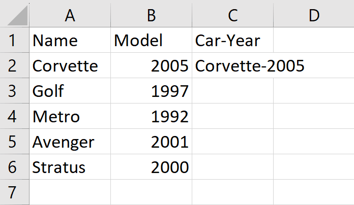
Step 5 – Apply the function on the complete column

- After getting the result on the first cell, drag the cell till the last cell contains names
Method 2: Combine cells separated with a dash using the Ampersand Operator with Array formula
In this method, we’ll use a simple Ampersand operator to combine cells but we’ll also convert the simple formula into an array formula which will tell Excel to apply the same formula to the complete range. So, follow along the steps explained below to learn how to achieve this goal.
Step 1 – Select the cell

- Click on the cell where you want to combine the names
Step 2 – Type the Formula
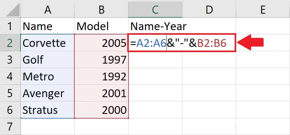
- After selecting the cell, type the formula as follows,
=A2:A6&“-”&B2:B6
In this formula, we have used Ranges A2:A6 and B2:B6, which tells Excel that we want to use an array formula.
Step 3 – Press the Enter key
- After typing the formula, press the Enter key to get the required result quickly
Method 3: Combine cells separated with a dash using the TEXTJOIN function
The TEXTJOIN function in Excel is used to join text from multiple cells or ranges, separated by a delimiter, into a single cell.
TEXTJOIN(delimiter, ignore_empty, text1, [text2], …)
- delimiter: The character(s) to be used as the delimiter between the text strings. This argument is required.
- ignore_empty: A logical value that specifies whether to ignore empty cells. This argument is also required.
- text1: The first text string or range to join. This argument is required.
- [text2], …: Additional text strings or ranges to join.
Step 1 – Select the cell
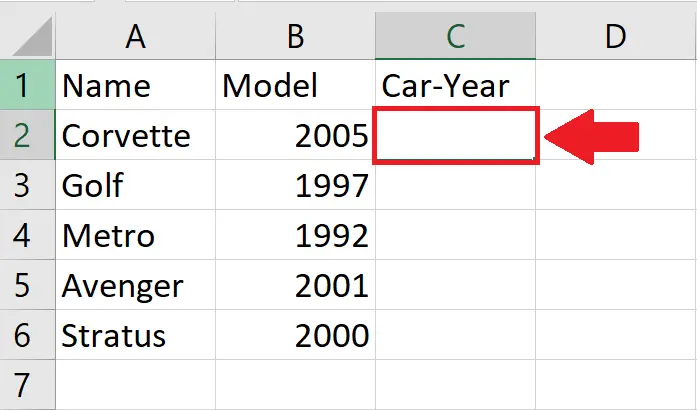
- Click on the cell where you want to combine the names
Step 2 – Use the TextJoin Function
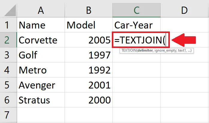
- After selecting the cell, type the TextJoin Function by typing “=TEXTJOIN(”
Step 3 – Type the Argument of the function
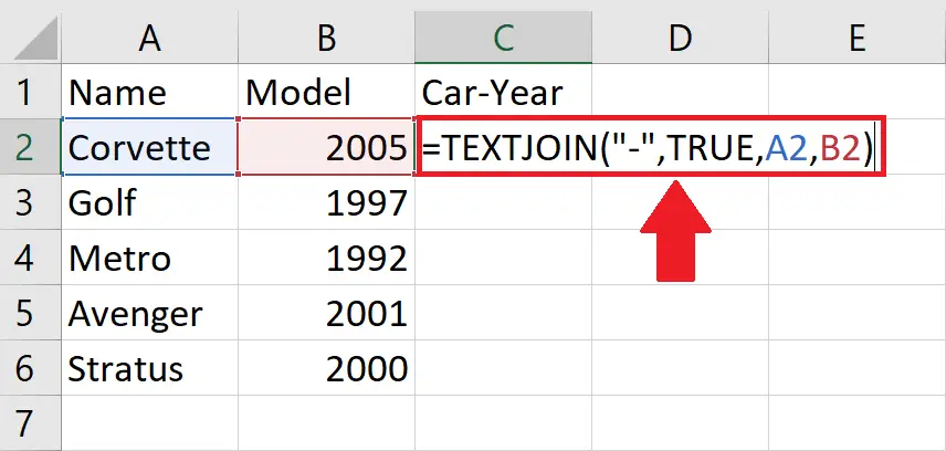
- Type the argument of the function as follows:
Delimiter: “-”
Ignore_empty: True
Text1: A2
Text 2: B2
Step 4 – Press the Enter key
- After typing the formula, press the Enter key to get the required result
Step 5 – Apply the function on the complete column
- After getting the result on the first cell, drag the fill handle till the last cell to apply the formula to every cell in the data range.
Method 4: Combine cells separated with a dash using the CONCATENATE function
The CONCATENATE function in Excel is used to join two or more strings of text into a single cell. The syntax for the CONCATENATE function is as follows:
=CONCATENATE(text1, [text2], …)
Where:
- text1 is the first string of text you want to join.
- text2 (optional) is the second string of text you want to join.
Step 1 – Select the cell

- Click on the cell where you want to combine the cells
Step 2 – Use the CONCATENATE Function
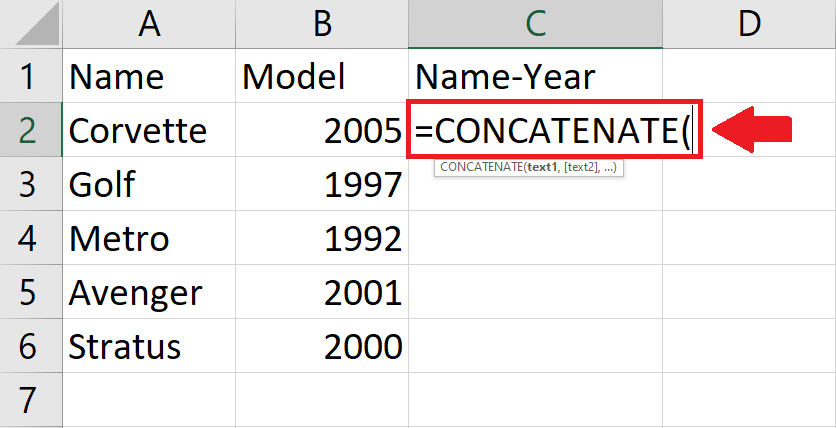
- After selecting the cel, use the CONCATENATE function by typing “=CONCATENATE(”
Step 3 – Type the Arguments of Function
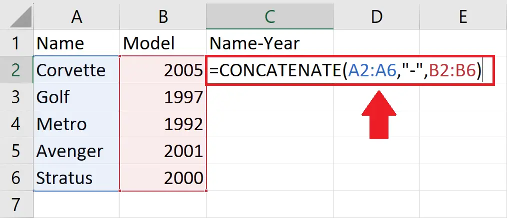
- After typing the CONCAT function, type the arguments as follows:
- Text 1: A2:A6
- After text 1, type “-”
- Text 2: B2:B6
- After typing the arguments, type a closing bracket “)”
Step 4 – Press the Enter key
- After typing the arguments, press the Enter key to get the required result


