
How to combine names in Excel
 By
SpreadCheaters
By
SpreadCheaters
This feature allows users to join the data from different cells. It does not depend upon the symmetry of data. Users can easily combine data from different cells.
To do this we have a built-in function of textjoin. To understand the usage of this function, let’s explore an example with steps.
Microsoft Excel has a lot of built-in functions for the ease of users. As Excel gives us the ability of data manipulation, likewise, there is another tremendous feature of Excel which will be used to combine the text data.
Step 1 – Select the cell
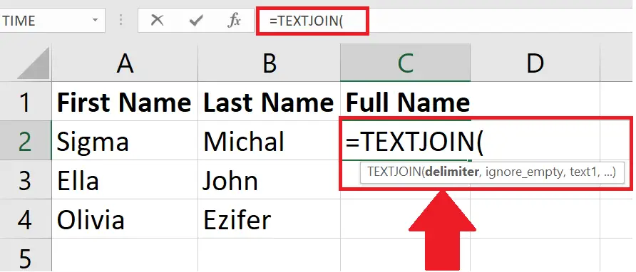
– Select a blank cell where you wish to join the data from different cells. In this case the selected cell is C2.
Above is a picture with an example.
Step 2 – Apply formula

– In the desired cell apply formula, The formula is given below;
=textjoin(delimiter, ignore_empty , text1, text2 ,…)
delimiter: The delimiter will be the special character inside inverted commas “ ” to separate the text. We’ll use the “,”.
Ignore_empty: It is a Boolean (true/false) value. It decides if the empty cells are to be included or not.
text1, text2: these will be the text values from different cells to be combined.
– Now, select the first, second and third value from the cells you wish to join.
– As soon as you press the enter key, the text will be joined and displayed in the desired selected cell.
Hence, names from different cells have been joined. Hence, using the TEXTJOIN function we can merge more than one cell’s data in a single cell with desired delimiter.


