How to combine 2 graphs in Excel

Combining two graphs in Excel means overlaying or displaying two or more charts or graphs on the same chart sheet or axis. It enables you to compare multiple data sets, identify trends and correlations, and present your data in a more comprehensive and visually appealing manner. By saving time and space, it helps to improve the efficiency and effectiveness of data analysis. 

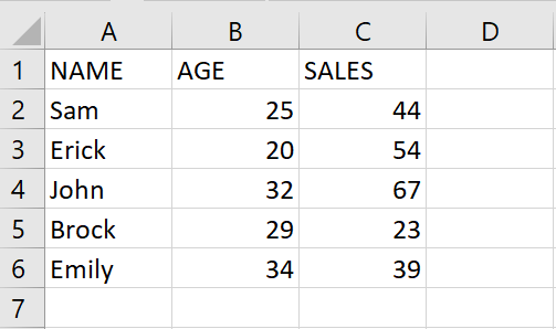
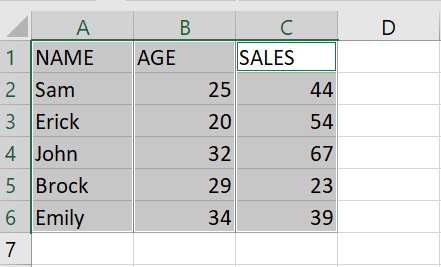
Our dataset includes the names of employees, their ages, and the number of sales they made in a month. This data will be used to create two separate charts: the first chart will display names and ages, while the second chart will display names and sales. To combine these charts, we have two methods i.e. by using Copy and paste option and by Using the combo chart option.

Method 1: Combine Charts using Copy and Paste option

Step 1 – Select the range of cells

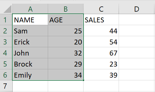
• Select the range of cells for which you want to form the first graph

Step 2 – Click on the Insert tab

• After selecting the range of cells, click on the Insert tab from the taskbar

Step 3 – Click on the Insert Line or Area Chart option

• From the Charts group of the Insert tab, click on the Insert Line or Area Chart option and the chart of the selected data will appear on the sheet

Step 4 – Select a range of cells

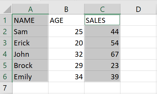
• Select the range of cells for the second chart
• To select the two nonadjacent columns select the cells of the first column and press Enter key, while pressing the Enter key select the cells of the second column

Step 5 – Click on the Insert Line or Area Chart option

• From the Charts group of the Insert tab, click on the Insert Line or Area Chart option and the chart of the selected data will appear on the sheet

Step 6 – Copy the Graph

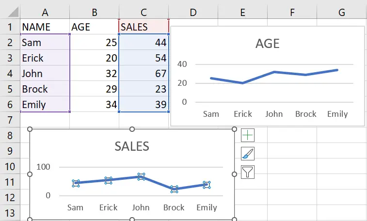
• Click on the Graph line of the second graph to select it
• After selecting it press CTRL+C to copy it 

Step 7 – Paste the Graph line

• After copying the graph line of the second graph, click on the first graph to select it
• After selecting the first graph, press CTRL+V to get the required result

Method 2: Combine charts using the Combo Charts option

Step 1 – Select the range of cells

• Choose the cells in the column that will be displayed in both charts.
• Hold down the CTRL key.
• Select the cells in the column that match the values in the first chart.
• Select the cells in the column that match the values in the second chart.

Step 2 – Click on the Recommended Chart option

• After selecting the range of cells, click on the Recommended Chart option and a dialog box will appear 

Step 3 – Click on the All Charts option

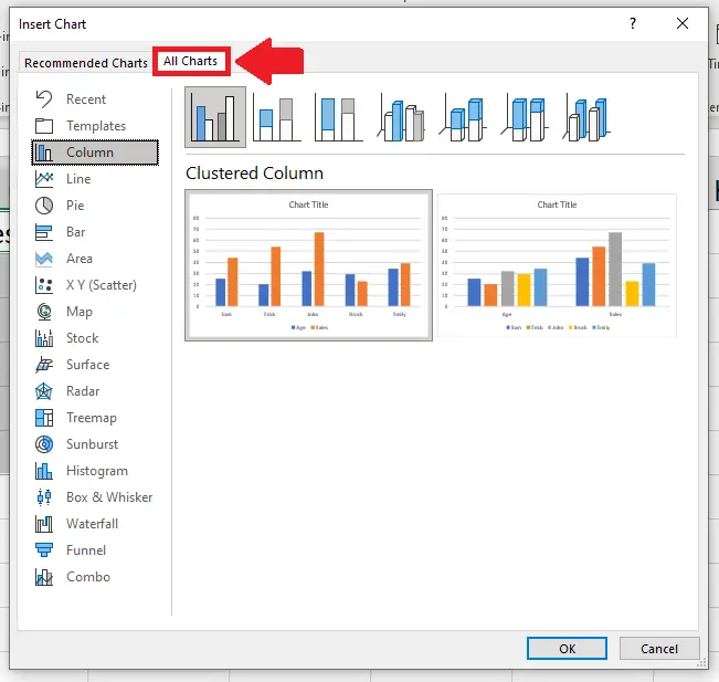
• In the dialog box, click on the All Charts option at the top of the dialog box and a list of options will appear

Step 4 – Click on the Combo option

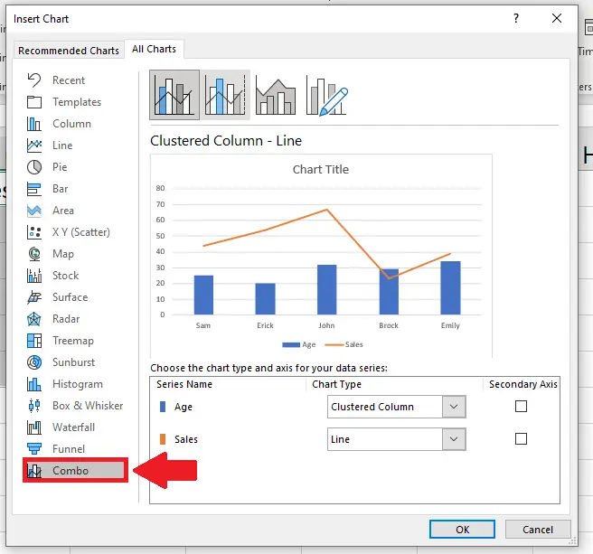
• From the dialog box, click on the Combo option 

Step 5 – Select the Type of Graphs

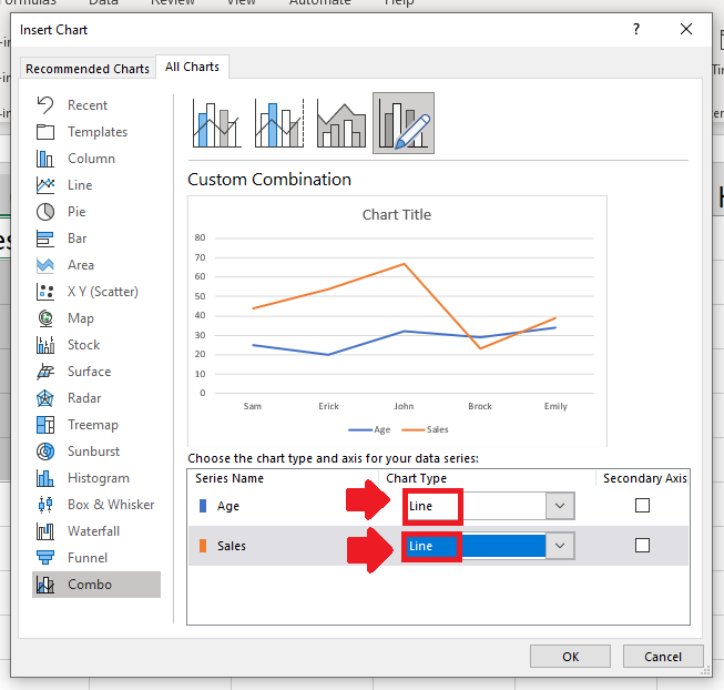
• From the dialog box, select the type of graphs you want to combine
• Here we have selected line graphs you may select any other type of graph

Step 6 – Click on the Okay option

• After selecting the type of graph, click on the OK option to get the required result