
How To Colour Cell Based On Value In Excel
 By
SpreadCheaters
By
SpreadCheaters
When we work with a huge amount of data in Excel and need to highlight or colour certain cells based on their values then it becomes very difficult to perform this task by changing the colour of each cell one by one. Colouring the cells based on their values in Excel helps in understanding the data and highlights the important data from the remaining cells.
Excel is an easy-to-use tool that helps its users by providing so many different methods for processing and categorising data within a few minutes. The following methods of MS Excel’s built in features will help you understand How to colour cells based on value in Excel.
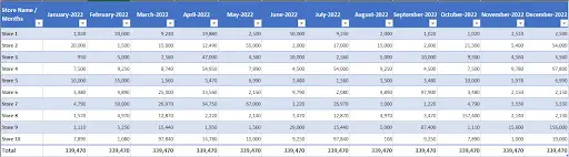
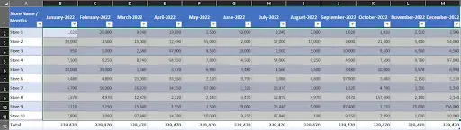
Let’s assume that we have sales data of 10 stores & we want to highlight cells based on their values.
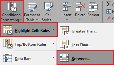
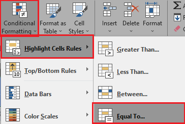
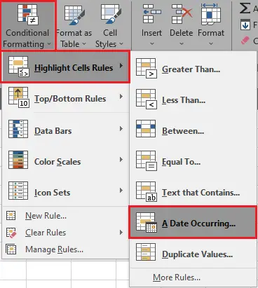
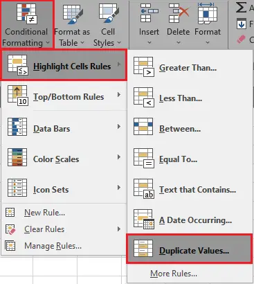
Step 1 – Select Conditional Formatting
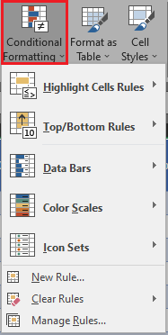
- Click on the conditional formatting button in the Home Tab. It will show different options, as shown above.
Step 2 – Go To Highlight Cell Rules
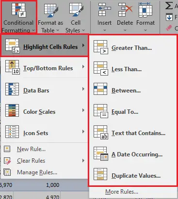
- Move your cursor to Highlight Cell Rules. It will show 07 options. Let’s explore these options one by one.
Method 1 – Highlight Cell Rules → Greater Than
Step 1 – Select Data Range

- With the help of the selection handle, select data in the table.
Step 2 – Go To Highlight Cell Rules
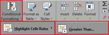
- Select > Greater Than option.
Step 3 – Set Condition & Cell Formatting
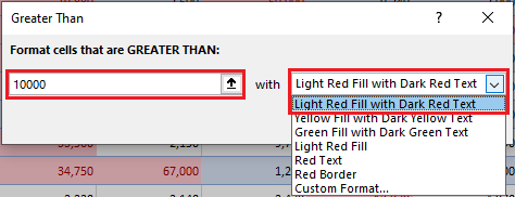
- Let’s assume that we want to highlight cells having sales value greater than 10,000.
- We will type 10,000 as condition & select desired cell formatting. We are choosing the default cell formatting i.e Light Red Fill with Dark Red Text.
- Click the OK button.
Step 4 – Get the Cells Highlighted With the Given Condition
- You will notice that after applying the condition, data in your table will be highlighted.
Method 2 – Highlight Cell Rules → Less Than
Step 1 – Select Data Range

- With the help of a selection handle, select data in the table.
Step 2 – Go To Highlight Cell Rules
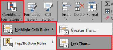
- Select < Less Than option.
Step 3 – Set Condition & Cell Formatting
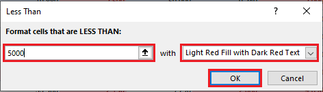
- Now we want to highlight all the cells having sales value less than 5,000. We will type 5,000 as condition & select desired cell formatting.
- Click the OK button.
Step 4 – Get the Cells Highlighted With the Given Condition
- You will notice that after applying the condition, data in your table will be highlighted.
Method 3 – Highlight Cell Rules → Between
Step 1 – Select Data Range
- With the help of a selection handle, select data in the table.
Step 2 – Go To Highlight Cell Rules
- Select Between option.
Step 3 – Set Condition & Cell Formatting
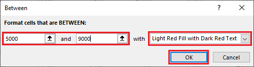
- Now we want to highlight all the cells having sales value between 5,000 to 9,000. Type 5,000 & 9,000 as lower & upper values & select desired cell formatting.
- Click the OK button.
Step 4 – Get the Cells Highlighted With the Given Condition

- You will notice that after applying the condition, data in your table will be highlighted.
Method 4 – Highlight Cell Rules → Equal To
Step 1 – Select Data Range

- With the help of a selection handle, select data in the table.
Step 2 – Go To Highlight Cell Rules
- Select Equal To option.
Step 3 – Set Condition & Cell Formatting
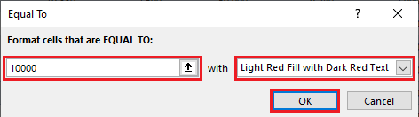
- Now we want to highlight all the cells having sales value equal to 10,000. Type 10,000 as condition & select desired cell formatting.
- Click the OK button.
Step 4 – Get the Cells Highlighted With the Given Condition
- You will notice that after applying the condition, data in your table will be highlighted.
Method 5 – Highlight Cell Rules → Text That Contains
Step 1 – Select Data Range

- With the help of a selection handle, select data in the table.
Step 2 – Go To Highlight Cell Rules
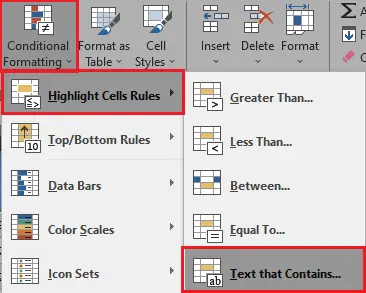
- Select Text That Contains option.
Step 3 – Set Condition & Cell Formatting
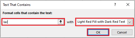
- Type lac as condition & select desired cell formatting.
- Click the OK button.
Step 4 – Get the Cells Highlighted With the Given Condition
- You will notice that after applying the condition, data in your table will be highlighted.
Method 6 – Highlight Cell Rules → A Date Occuring
Step 1 – Select Data Range
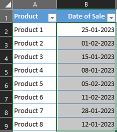
- With the help of a selection handle, select data in the table.
Step 2 – Go To Highlight Cell Rules
- Select A Date Occuring option.
Step 3 – Set Condition & Cell Formatting
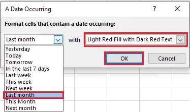
- Select Last month from the drop down list as condition & select desired cell formatting.
- Click the OK button.
Step 4 – Get the Cells Highlighted With the Given Condition
- You will notice that after applying the condition, data in your table will be highlighted.
Method 7 – Highlight Cell Rules → Duplicate Values
Step 1 – Select Data Range
- With the help of a selection handle, select data in the table.
Step 2 – Go To Highlight Cell Rules
- Select Duplicate Values option.
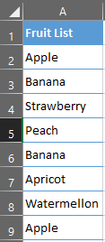
Step 3 – Set Condition & Cell Formatting
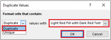
- We want to find duplicate fruit names in the list so, select Duplicate from the drop down list & select desired cell formatting.
- Click the OK button.
Note: Similarly, if you want to highlight unique values from the list. Select Unique from the drop down list.
Step 4 – Get the Cells Highlighted With the Given Condition
- You will notice that after applying the condition, data in your table will be highlighted.


