How to color code rows in Excel

Color coding rows in Excel means using different background colors to visually differentiate between rows that have different characteristics or properties. Color coding rows in Excel is an important technique that helps to improve the readability, organization, and analysis of data. It allows users to easily identify and understand critical data points, leading to better decision-making and improved productivity.

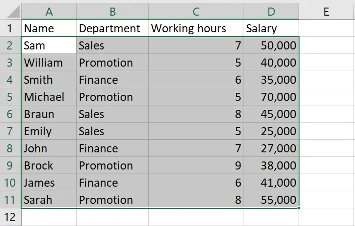
We have a dataset that contains information about the employees of a company, including their names, salaries, and working hours. To visually differentiate between rows that have different characteristics or properties, we want to color code the rows based on certain conditions. To achieve this, we will select the range of our data and then apply various New Rules in Conditional Formatting based on our specific requirements, to obtain the desired result.

Method 1: Color code the rows based on Equal condition

Step 1 – Select the range of cells

• Select the range of cells from which you want to color the rows

Step 2 – Click on the Conditional Formatting option 

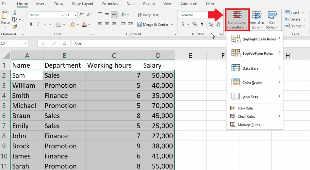
• After selecting the range of cells, click on the Conditional Formatting option and a drop-down menu will appear

Step 3 – Click on the New Rule option

• From the drop-down menu, click on the New Rule option and a dialog box will appear

Step 4 – Click on the Use a Formula

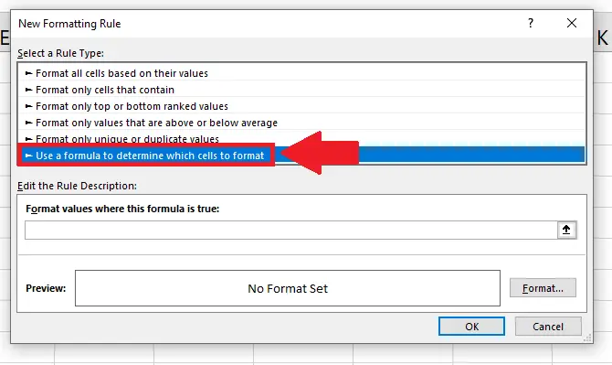
• From the dialog box, click on the Use a Formula to determine which cells to format option, and a dialog box will appear

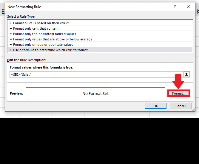
Step 5 – Type the Formula

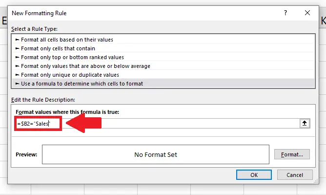
• In the dialog box, type the following formula in the box below the Format values where this formula is true option:
• =$B2=“Sales”

Step 6 –  Click on the Format option

• In the dialog box, click on the Format option and a dialog box will appear

Step 7 – Select the Color 

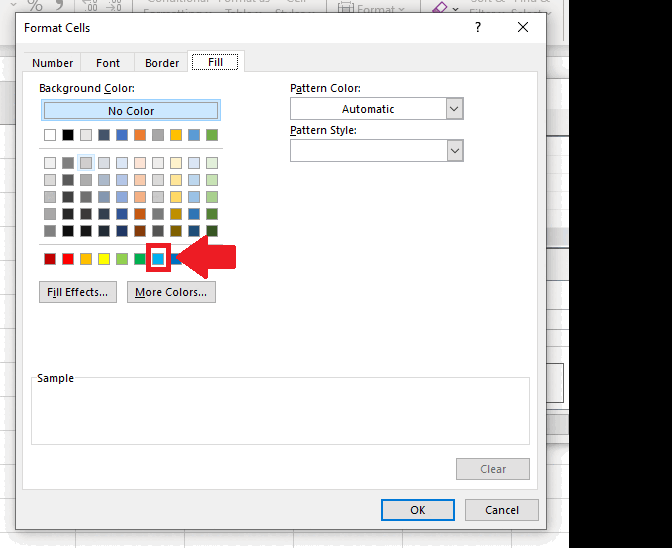
• From the dialog box, click on the color you want and then click on the OK option at the end of the dialog box and the color will appear on the last dialog box

Step 8 – Click on the OK option

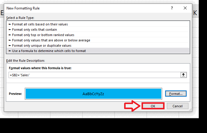
• Click on the OK option to get the required result

Method 2: Color code the rows by using the Less/Greater than the condition

Step 1 – Set the Reference value

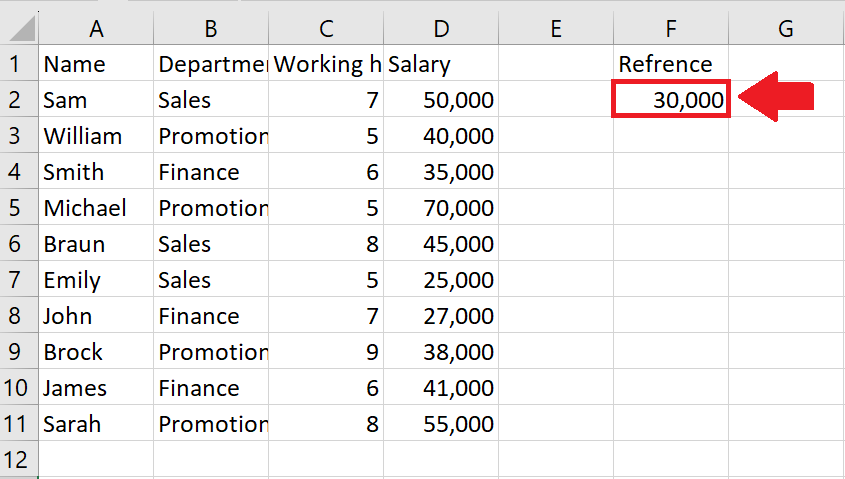
• Set the reference value to less than what you want to color

Step 2 – Select the range of cells

• Select the range of cells from which you want to color the rows

Step 3 – Click on the Conditional Formatting option 

• After selecting the range of cells, click on the Conditional Formatting option and a drop-down menu will appear

Step 4 – Click on the New Rule option

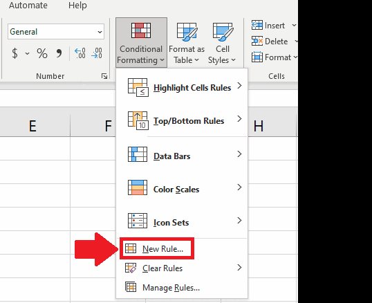
• From the drop-down menu, click on the New Rule option and a dialog box will appear

Step 5 – Click on the Use a Formula

• From the dialog box, click on the Use a Formula to determine which cells to format option, and a dialog box will appear

Step 6 – Type the Formula

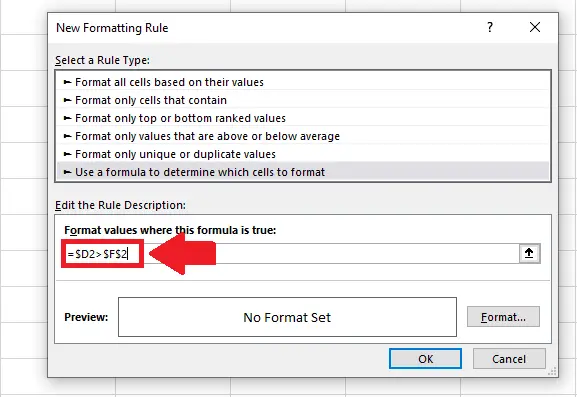
• In the dialog box, type the following formula in the box below the Format values where this formula is true option:
• =$D2>$F$2

Step 7 –  Click on the Format option

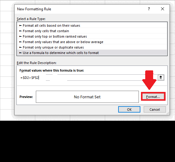
• In the dialog box, click on the Format option and a dialog box will appear

Step 8 – Select the Color 

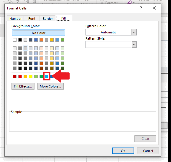
• From the dialog box, click on the color you want and then click on the OK option at the end of the dialog box and the color will appear on the last dialog box

Step 9 – Click on the OK option

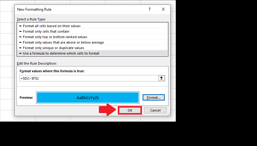
• Click on the OK option to get the required result