
How to color cells in Excel based on value
 By
SpreadCheaters
By
SpreadCheaters

Microsoft Excel offers a very interesting way to color cells based on a value. We can cater to this problem statement by using the “conditional formatting” option. We can perform the below mentioned way to color cells based on a value in excel:
We’ll learn about this methodology step by step.
To do this yourself, please follow the steps described below;
Step 1 – Excel sheet with a column filled with numbers

– Open the desired Excel workbook containing a column with numbers
Step 2 – Conditional formatting
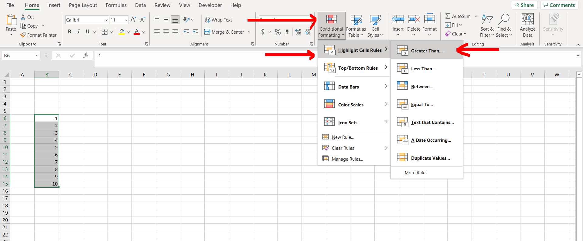
– Now select the cells containing the numbers and then under the Home option in the menu bar, click on “Conditional Formatting”, and then select “Highlight cell rules”, and then select any one of the available options. We have chosen “Greater than”, as we can see in the image above.
Step 3 – Entering the condition
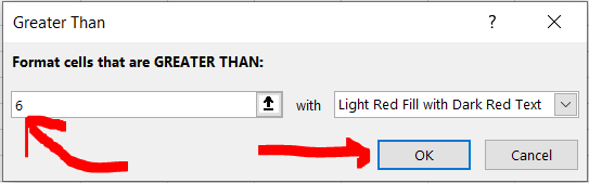
– Now type in the number, greater than which cells will be colored, and then click “OK”.
Step 4 – Cells colored
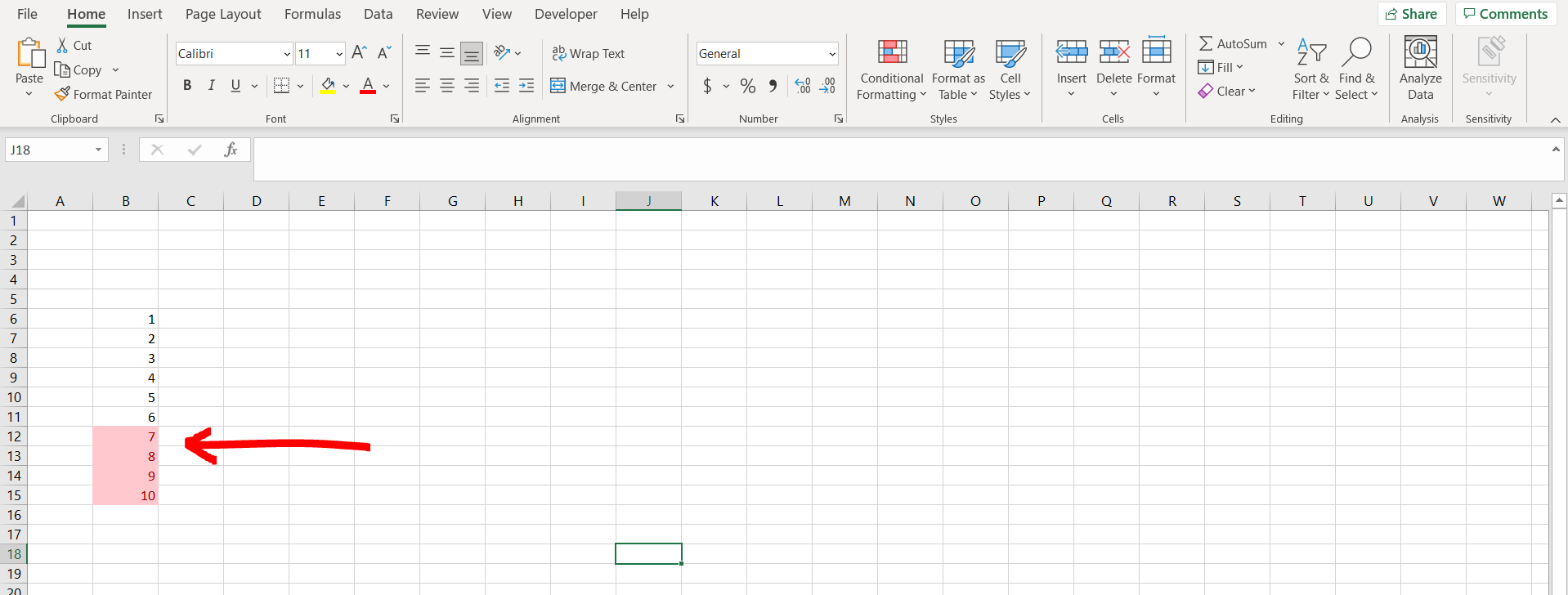
– We can see that the cells which are greater than “6” have been colored


