
How to collapse rows in a pivot table in Excel
 By
SpreadCheaters
By
SpreadCheaters
You can watch a video tutorial here.
Pivot tables are one of the most useful tools in Excel for summarizing and analyzing data. Pivot tables are built off a table or a dataset and can summarize rows or columns. When you want to collapse rows, you can add another field that groups the rows, to the pivot table structure. This will automatically group the rows and you can then collapse or expand the rows as needed.
Step 1 – Open the Field List
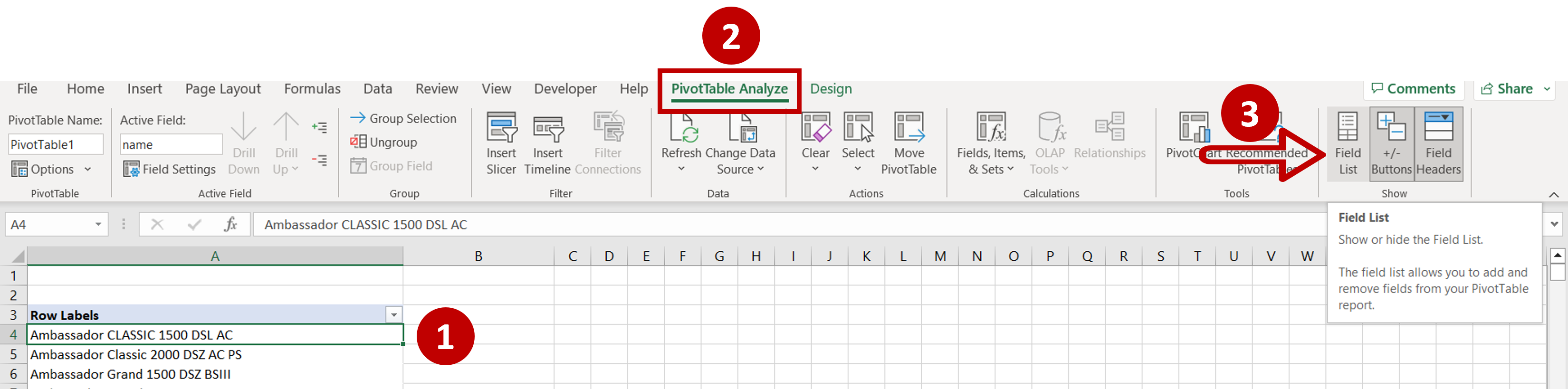
– Select any cell in the pivot table
– Go to PivotTable Analyze > Show
– Click on the Field List button
Step 2 – Add another field to the rows section
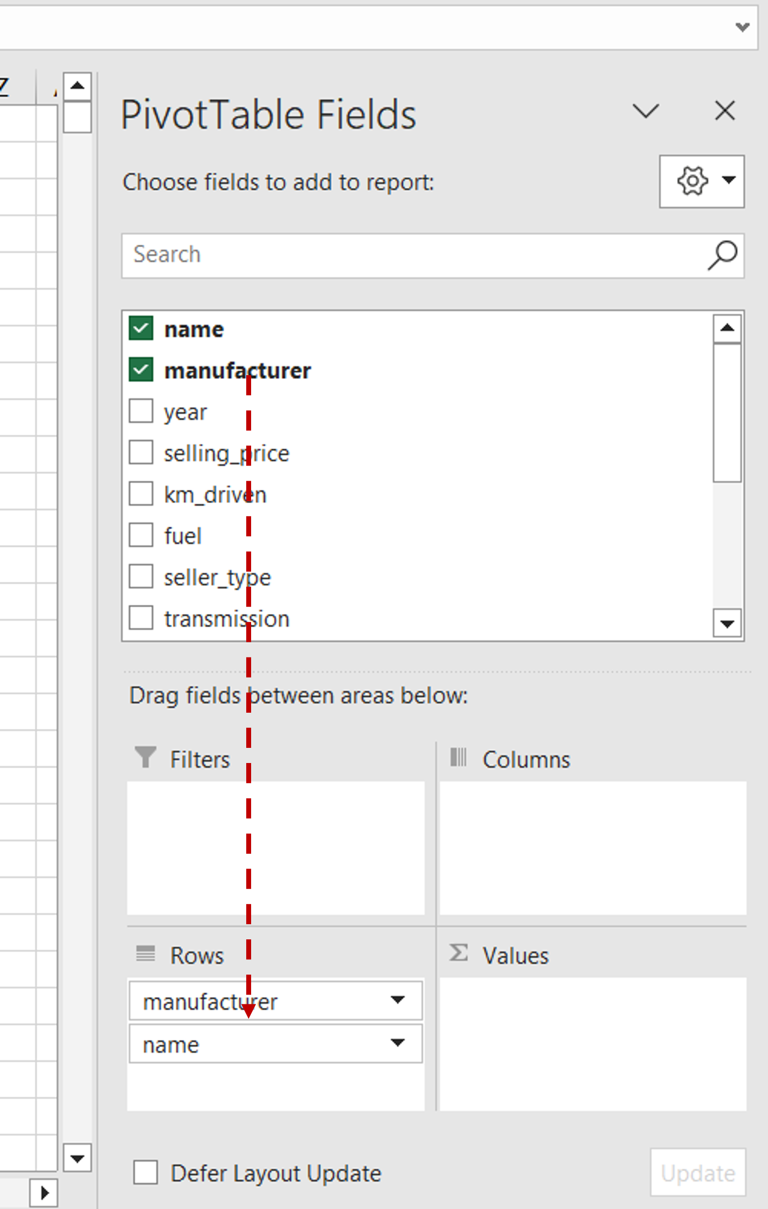
– Drag the ‘manufacturer’ field to the Rows section above ‘name’
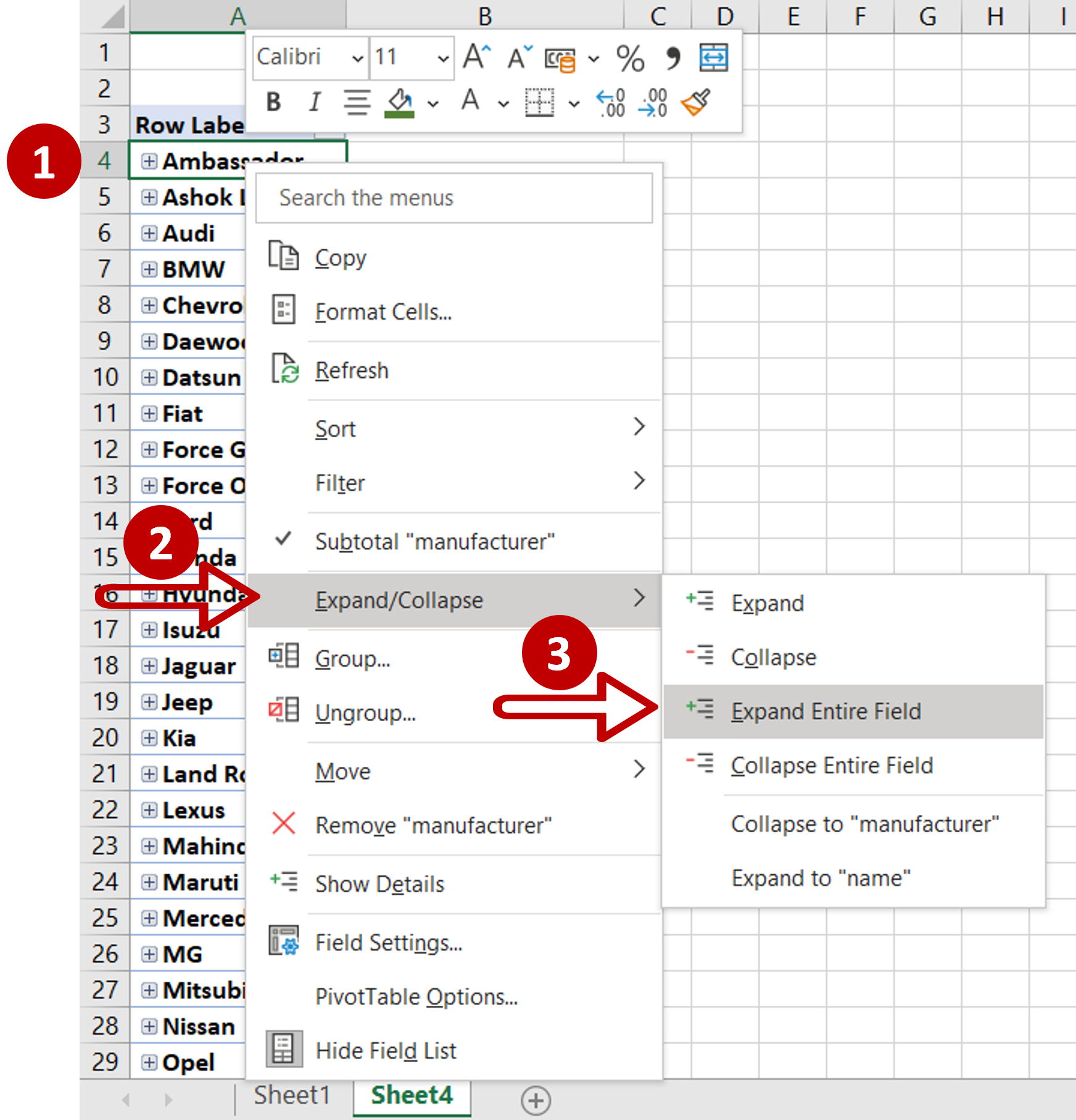
Step 3 – Expand the rows
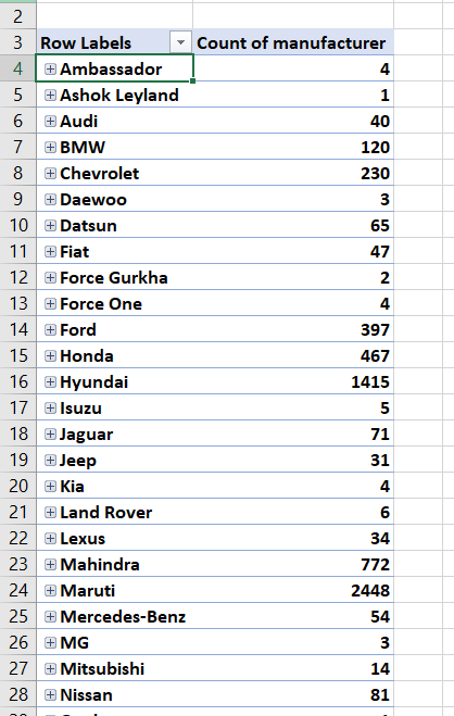
– The rows are collapsed
– Select any row in the table
– Right-click and expand the Expand/Collapse section
– Choose Expand Entire Field
Step 4 – Check the result
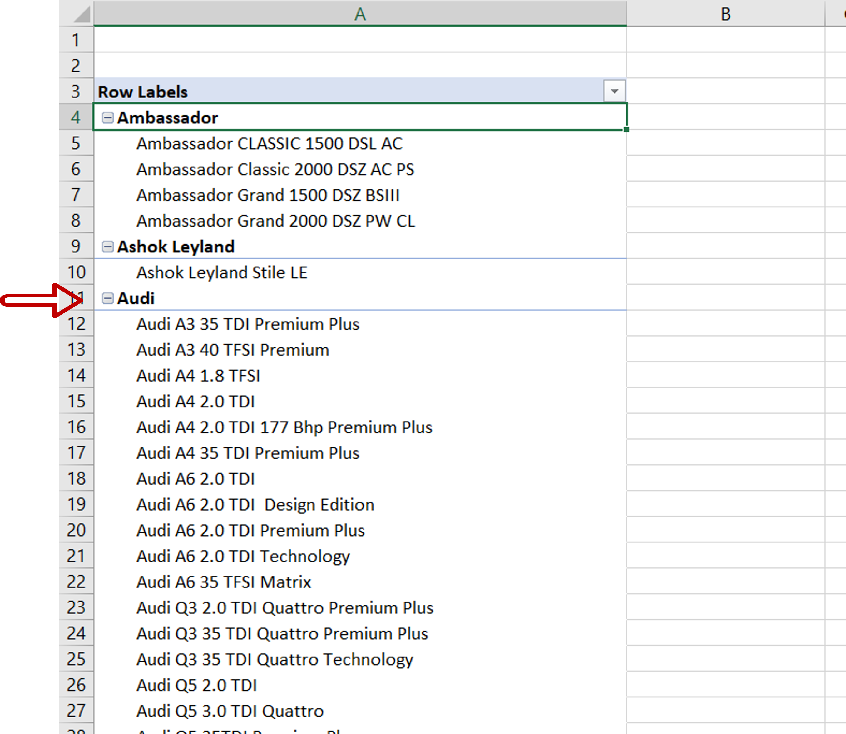
– The rows can be collapsed or expanded


